< HOME > 10-10-2022 WEATHER CONTROL - First Steps ... > working with Japanese PhDs - to make weather control product
Source: https://a.tellusjournals.se/article/10.3402/tellusa.v67.24216/ SHRED by Susan ... added, clarified ( ... )
Dynamic Meteorology > https://www.sciencedirect.com/topics/earth-and-planetary-sciences/dynamic-meteorology
"... Overview: J.R. Holton, in Encyclopedia of Atmospheric Sciences (Second Edition), 2015
( https://www.sciencedirect.com/referencework/9780123822253/encyclopedia-of-atmospheric-sciences )
Introduction: "Dynamic meteorology" is the branch of fluid dynamics [ https://en.wikipedia.org/wiki/Fluid_dynamics ] concerned with the meteorologically significant motions of the atmosphere. [ https://en.wikipedia.org/wiki/Meteorology ] ...
It (meteorology) forms the primary scientific basis for weather and climate prediction, and thus plays a primary role in the atmospheric sciences. Most of the meteorologically important motions studied in dynamic meteorology are profoundly influenced by the facts that the Earth is a rapidly rotating planet, and that the atmosphere (of the earth) on average has "stable density stratification".
[ http://maeresearch.ucsd.edu/linden/MAE/ch3_04.pdf - page 3 ]
These facts (above) make the "fluid dynamics" of the (earth's) atmosphere very different from traditional engineering fluid dynamics.
Planetary rotation places strong "constraints" on large-scale horizontal motions (east to west to east); stable stratification places strong constraints on vertical motions (north to south to north). These constraints can be understood - by considering the fundamental physical laws governing motions of the atmosphere.
The motions of the (earth's) atmosphere are governed by the laws for conservation of mass, conservation of momentum, and conservation of thermodynamic energy.
( https://www.youtube.com/watch?v=_9bGKi3iX5Q :
https://openclimate.org/course-collection-introduction-to-dynamical-meteorology-climate-earth-401-u-m/ )
Application of these laws to motions with horizontal scales of several hundred kilometers or greater leads to simple relations among the horizontal wind, pressure, and temperature distributions.
[For Americans: there are approximately three (3) feet in a meter; A kilometer is one thousand meters- about three thousand feet; - thus, several hundred kilometers is equivalent to "several hundred" thousand times three feet - which is ... A "mile" in "feet" = 5,280 feet.
NOTE: The diameter of the eye of hurricane Ian ( at US land fall) was 26 miles ...
3 feet x 1,000 = 3000 feet x "several hundred" > 300,000 feet object ( https://en.wikipedia.org/wiki/K%C3%A1rm%C3%A1n_line < Kármán line )
https://www.nasa.gov/image-feature/staring-into-the-hurricanes-eye :
Source: https://www.universetoday.com/157934/gaze-down-into-the-eye-of-hurricane-ian-seen-from-orbit/ ..."... The natural-color image above was acquired by the satellite’s Operational Land Imager camera at 11:57 a.m. local time (15:57 Universal Time), three hours before the storm made landfall in Caya Costa, Florida. At the time the image was taken, the eye was 42 kilometers (26 miles) in diameter. ..." ] ... These relations form a set of diagnostic relations essential for understanding the motions that generate weather disturbances. [ IBM "diagnostic analysis"
: https://research.ibm.com/publications/diagnostic-analysis-directional-relation-graph ]
Such motions are generally rotational in character. They can be characterized by a conservable property known as the potential vorticity, which is the fluid dynamical analogue of spin angular momentum in solid mechanics ... [ https://rammb.cira.colostate.edu/wmovl/vrl/tutorials/satmanu-eumetsat/satmanu/basic/parameters/pv.htm ]
[ longitude latitude > https://en.wikipedia.org/wiki/Geographic_coordinate_system ]
The "latitudinal gradient" of "potential vorticity" provides the mechanism for generation of global-scale planetary waves, which are primary features of the climate system.
[ https://www.sciencedirect.com/topics/earth-and-planetary-sciences/dynamic-meteorology ]
Superposed on these global waves are transient cyclones and anticyclones, whose energy is derived primarily from the potential energy associated with the mean Pole-to-Equator temperature gradient. ... Study of the development and evolution of transient weather disturbances, and of dynamical mechanisms for producing intraseasonal and interannual climate variations, are among the principal areas of study in dynamic meteorology. ..."
Americans - such as Susan - get involved
- because these Americans - were told as children - [that] - there is NOTHING [that] "Americans" cannot do. The practicality and expense - is another matter...
[ SOURCE: https://a.tellusjournals.se/article/10.3402/tellusa.v67.24216/ ]
" Thermodynamics of a tropical cyclone:
generation and dissipation of mechanical energy in a self-driven convection system "
Authors:
Hisashi Ozawa ( https://home.hiroshima-u.ac.jp/hozawa/index.html : Hiroshima University )
[ https://seeds.office.hiroshima-u.ac.jp/profile/en.145c27b265d5d890520e17560c007669.html ]
Shinya Shimokawa ( https://indico.in2p3.fr/event/2481/contributions/24352/attachments/19647/24096/poster-A0.pdf )
Torus-04.JPG - Torus-01.JPG
Tropical-CyClone-02.JPG
Torus-03.JPG
Torus-02.JPG
Tropical-CyClone-01-new-with-tropopause-arrow-gone.jpg
In this article:
( Abstract )
1. Introduction
2. Thermodynamic equations
3. Tropical cyclones
4. Discussion and conclusion
Acknowledgements
Footnotes
References
NOTE: American ENGLISH speakers & AMERICANS refer to a tropical cyclone - as a "Hurricane" . ( https://www.nhc.noaa.gov/ )
"Everyone talks about the weather - no one does anything about the weather" ... - Charles Dudley Warner & Mark Twain
If you want something "explained" - hire an American women - who knows absolutely nothing about it; Over-pay her! and tell her [that] she will be responsible for "teaching it" - to a room filled with eigth graders - in the bottoms area of Columbus, Ohio. - GREAT RESULTS - EVERY TIME !
Abstract [ SOURCE: https://a.tellusjournals.se/article/10.3402/tellusa.v67.24216/ ]
The formation process of circulatory motion of a tropical cyclone is investigated from a thermodynamic viewpoint. The generation rate of mechanical energy by a fluid motion under diabatic heating and cooling, and the dissipation rate of this energy due to irreversible processes are formulated from the first and second laws of thermodynamics. This formulation is applied to a tropical cyclone, and the formation process of the circulatory motion is examined from a balance between the generation and dissipation rates of mechanical energy in the fluid system. We find from this formulation and data analysis that the thermodynamic efficiency of tropical cyclones is about 40% lower than the Carnot maximum efficiency because of the presence of thermal dissipation due to irreversible transport of sensible and latent heat in the atmosphere. We show that a tropical cyclone tends to develop within a few days through a feedback supply of mechanical energy when the sea surface temperature is higher than 300 K, and when the horizontal scale of circulation becomes larger than the vertical height of the troposphere. This result is consistent with the critical radius of 50 km and the corresponding central pressure of about 995 hPa found in statistical properties of typhoons observed in the western North Pacific.
1. Introduction [ SOURCE: https://a.tellusjournals.se/article/10.3402/tellusa.v67.24216/ ]
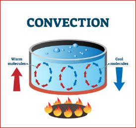
A "tropical cyclone" is a large-scale convection system driven by a temperature contrast between the hot tropical sea surface and the cold top of the troposphere and is characterised by a low-pressure centre and inward spiral convergence of strong winds towards the centre.
The typical diameter is from 200 to 2000 km, wind speed is from 20 to 85 m s−1 and the typical central pressure generally ranges from 990 to 870 hPa, corresponding to central pressure drops of 20–140 hPa. As a conventional classification, tropical cyclones with maximum wind speeds larger than 33 m s−1 are called typhoons in the western North Pacific, hurricanes in the eastern North Pacific and western North Atlantic and severe tropical cyclones in other regions. A comprehensive review on this subject can be found in the articles by Bergeron (1954) and Emanuel (2003).
convective-motion-02.JPG
convective-motion-01.JPG 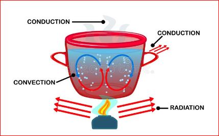
convective-motion-03.JPG  hhh
hhh
h
Tropical-CyClone-01-new-with-tropopause-arrow-gone.jpg ![]()
Figure 1 shows a schematic cross-section of a tropical cyclone. ... The air is heated at the sea surface with temperature T s and is cooled at the top of the troposphere with temperature T t. The heated air is ascending at the centre, and the cooled air is descending in the margin, thereby forming a circulatory motion.
[ In 3-dimensions - the system is a torus.
Torus-05.JPG 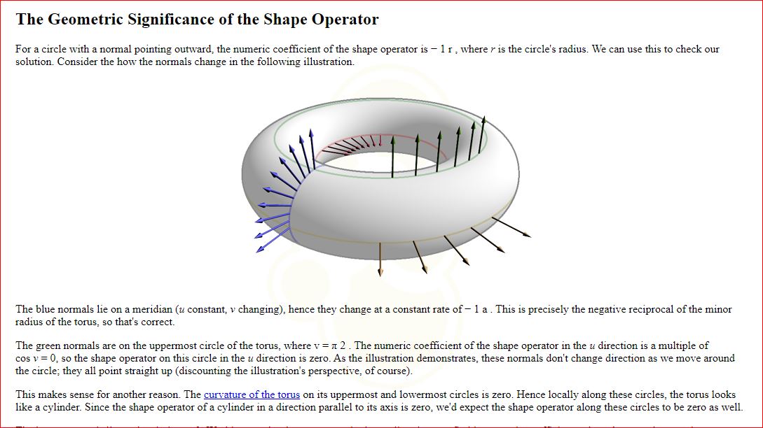
Torus-04.JPG 
Torus-03.JPG
Torus-02.JPG
Torus-01.JPG 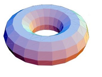 Torus-01.JPG
ring-toss-04.JPG 
ring-toss-03.JPG 
ring-toss-02.JPG 

Tropical-CyClone-01-new-with-tropopause-arrow-gone.jpg ![]() HHHHH
HHHHH
As shown in the figure, there is a large-scale circulatory motion of air in this system, with a convergence of the air mass near the sea surface and a divergence of the air mass at the upper troposphere.
Both the sea-level convergence and upper-level divergence are associated with an ascending motion at the centre, and a descending motion at the margin (sides) , respectively, thereby closing the circulation.
Through this circulation, the air is heated at the hot sea surface and is cooled at the top of the troposphere. With the heating and cooling processes, the air expands near the sea surface with a supply of water vapour, and it contracts in the upper troposphere, with the water vapour condensing to precipitation.
Since expansion takes place near the sea surface where the pressure is high, and contraction takes place in the upper troposphere where the pressure is low, part of the heat energy received at the sea surface is converted into mechanical work through the circulation of the atmosphere.
The "mechanical work" thus produced is stored in the "background gravitational field" as a ‘top-heavy’ density distribution that is gravitationally unstable.
( This can be demonstrated by a children's "ring toss" game.
(Strictly speaking, this is a potentially "top-heavy density distribution", whose instability could be realised if the atmosphere were in the isobaric condition.)
The maximum amount of mechanical energy that can be extracted from this potentially unstable state was investigated by Lorenz (1955, 1967) and is called available "potential energy".
Lorenz E. N . Available potential energy and the maintenance of the general circulation . Tellus . 1955 ; 7 : 157 – 167 .
[ https://eapsweb.mit.edu/sites/default/files/Available_Potential_Energy_1955.pdf ]
Lorenz E. N . The Nature and Theory of the General Circulation of the Atmosphere . 1967 ; Geneva : World Meteorological Organization .
[ http://users.uoa.gr/~pjioannou/historical/Lorenz-1967.pdf ]
Lorenz R. D. , Lunine J. I. , Withers P. G. , McKay C. P . Titan, Mars and Earth: entropy production by latitudinal heat transport . Geophys. Res. Lett . 2001 ; 28 : 415 – 418 .
Lorenz R. D. , Rennó N. O . Work output of planetary atmospheric engines: dissipation in clouds and rain . Geophys. Res. Lett . 2002 ; 29 : 1 – 4 .
Ozawa H. , Ohmura A. , Lorenz R. D. , Pujol T . The second law of thermodynamics and the global climate system: a review of the maximum entropy production principle . Rev. Geophys . 2003 ; 41 : 1018 . 1 – 24 .
Part of this available "potential energy" is converted into kinetic energy of the fluid motion, thereby sustaining the circulation. In a steady state, the kinetic energy is dissipated into heat (random thermal motion of molecules) by turbulent drag force in the atmosphere with the action of viscosity, and the energy conversion rate is balanced by the energy dissipation rate.
The remaining part of the available potential energy is dissipated directly through irreversible transport of sensible and latent heat in the atmosphere. This thermal dissipation process is known to exist in the atmosphere, and its contribution is estimated to be about 70% of the total energy dissipation in the global-scale atmospheric circulation (Pauluis and Held, 2002; Ozawa et al., 2003).
Thus, one can expect that the thermal dissipation also plays an important role in the energy conversion process in tropical cyclones.
While several studies have been carried out on the thermodynamic properties of tropical cyclones (e.g., Emanuel, 1986, 1987, 1999, 2003; Bister and Emanuel, 1998), the thermal dissipation process seems to have been missing from the previous work.
The purpose of this paper is therefore to investigate the thorough energy dissipation processes in a fluid system that exchanges energy with its non-equilibrium surroundings.
In this paper - we shall start with the basic laws of thermodynamics (the first and second laws), and present a set of equations [ 55 equations) that describe the generation and dissipation rates of mechanical energy in a fluid system. The derived equations are kept to be in a general form so that one can apply this method to any type of fluid system that interacts with its surroundings.
This method is applied to a tropical cyclone, and the formation process of the circulatory motion is examined from a balance between the generation and dissipation rates of mechanical energy. The relation of thermal and viscous dissipation to entropy production is also discussed.
Fig. 1 A schematic cross-section of a tropical cyclone. The air is heated at the sea surface with temperature T s and is cooled at the top of the troposphere with temperature T t. The heated air is ascending at the centre, and the cooled air is descending in the margin, thereby forming a circulatory motion.
In what follows, we present a set of equations that express the generation and dissipation rates of mechanical energy in a fluid system from the basic laws of thermodynamics (Section 2). These equations are applied to a tropical cyclone, and the formation process of the circulatory motion is examined in Section 3.
Results obtained from this study are examined and compared with the statistical properties of typhoons in the western North Pacific.
Implications of the results for general dynamical properties of non-linear non-equilibrium phenomena are discussed in Section 4.
2. Thermodynamic equations [ SOURCE: https://a.tellusjournals.se/article/10.3402/tellusa.v67.24216/ ]
2.1. First and second laws of thermodynamics
https://en.wikipedia.org/wiki/Thermodynamics
https://en.wikipedia.org/wiki/Laws_of_thermodynamics
https://en.wikipedia.org/wiki/Conservation_of_energy
https://en.wikipedia.org/wiki/Zeroth_law_of_thermodynamics
https://en.wikipedia.org/wiki/First_law_of_thermodynamics
https://en.wikipedia.org/wiki/Second_law_of_thermodynamics
https://en.wikipedia.org/wiki/Third_law_of_thermodynamics
"Entropy" > https://en.wikipedia.org/wiki/Entropy
...state of disorder, randomness, or uncertainty. ...
fluid system: ( https://geo.libretexts.org/Bookshelves/Meteorology_and_Climate_Science/Book%3A_Practical_Meteorology_(Stull)/01%3A_Atmospheric_Basics#:~:text=Meteorology%20is%20the%20study%20of,processes%20acting%20at%20different%20locations. )
convective motion: ( https://royalsocietypublishing.org/doi/10.1098/rspa.1940.0092 ) :: "On maintained convective motion in a fluid heated from below" byAnne Pellew & Richard Vynne Southwell Published:01 November 1940 " ( https://www.dreamstime.com/illustration/convective.html )
 ...
...
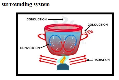
Let us first consider a fluid system in which convective motion will be produced and its surrounding system with which the fluid system exchanges heat energy.
Entropy of the fluid system and its surrounding system will be changed by the heat exchange process as well as by energy conversion processes in the fluid system.
Because of the additive properties of entropy, the entropy change of the whole system can be expressed as a sum of the entropy change in each system:
dSwhole = dSsys+dSsurr,
(1)
where dS whole, dS sys and dS surr represents the "entropy change" of the whole system, that of the fluid system and that of the surrounding system, respectively. The second law of thermodynamics states that all spontaneous processes proceed in the direction in which entropy of the whole (isolated) system increases:
dSwhole = dSsys+dSsurr≥0,
( 2 )
where the equality sign ( = ) refers to a reversible process with no net increase of entropy, a process that requires infinite time to proceed. All natural processes occur in a way that increases entropy in the whole system. This is a consequence of the second law of thermodynamics.
It should be noted that, since the entropy increase of the whole system is associated with irreversible processes, we can call the term dS "whole entropy production" due to irreversible processes that take place in the system.
It should be kept in mind, however, that "entropy production" is identical to the "net entropy increase" in the whole system, and this increase is a driving force for all spontaneous phenomena in nature.
We shall in due course discuss how this condition can account for the emergence of convective motion in a tropical cyclone.
"fluid parcel" > https://en.wikipedia.org/wiki/Fluid_parcel "...
In fluid dynamics, within the framework of continuum mechanics, a fluid parcel is a very small amount of fluid, identifiable throughout its dynamic history while moving with the fluid flow.[1] As it moves, the mass of a fluid parcel remains constant, while—in a compressible flow—its volume may change.[2][3] And its shape changes due to the distortion by the flow.[1] In an incompressible flow the volume of the fluid parcel is also a constant (isochoric flow).
This mathematical concept is closely related to the description of fluid motion—its kinematics and dynamics—in a Lagrangian frame of reference. In this reference frame, fluid parcels are labelled and followed through space and time. But also in the Eulerian frame of reference the notion of fluid parcels can be advantageous, for instance in defining the material derivative, streamlines, streaklines, and pathlines; or for determining the Stokes drift.[1]
The fluid parcels, as used in continuum mechanics, are to be distinguished from microscopic particles (molecules and atoms) in physics. ..."
Let us next consider that a small amount of heat energy is supplied from the surrounding system to a "fluid parcel" through the system boundary, where the absolute temperature T is assumed in a local equilibrium state.
In this case, the entropy of the surrounding system will decrease by
dSwhole = dSsys+dSsurr≥0,
(3)
where δ Q is the heat supplied from the surrounding system . [ δQ = heat supplied from the surrounding system.
The heat supplied to the fluid parcel (in the system) is changed partly into "internal energy" of the fluid parcel and partly into "mechanical work" by volume expansion of the heated fluid.
The internal energy of the "fluid parcel" will also be subject to volume expansion or contraction through the movement of the fluid parcel along its trajectory.
Moreover, the internal energy may be transferred to the surrounding cold fluid by heat conduction, thermal radiation, or by latent heat transport.
Suppose that all of this internal energy is finally transferred to the coldest region of the system with a minimum reference temperature T r. This reference temperature can be set to be that at the top of the troposphere (i.e., tropopause) T t in the case of a tropical cyclone (Fig. 1).
When the fluid expands at the system's surface where the temperature and pressure are high, and it contracts at the cold reference state where the pressure is low, part of the heat energy supplied to the fluid can be converted into mechanical work (δW=∫p dV≥0), even though the total volume change is zero, and the fluid parcel returns to the initial state (∫dV=0). The heat transferred to the reference state is then less than that gained at the system's surface, because of the first law of thermodynamics:
dSwhole=dSsys+dSsurr≥0,
(4)
where δQ′ is the heat transferred to the reference state, and δW is the mechanical work done by the fluid parcel. If we assume a cyclic return of the fluid parcel to the initial state, entropy of the fluid parcel remains unchanged. Entropy increase of the fluid system is then given by the heat transfer to the reference state divided by its temperature:
dSwhole=dSsys+dSsurr≥0,
(5)
Equation (5) implies that the conversion of heat into mechanical work reduces the entropy of the system, and therefore, an enormous amount of mechanical work conversion is prohibited by the second law [inequality; eq. (2)].
Substituting eqns. (3) and (5) into eq. (2), we can rewrite the second law as:
dSwhole=dSsys+dSsurr≥0,
(6)
The first term on the right-hand-side of the first equality denotes entropy increase by the heat transport from T to T r, and the second term denotes entropy reduction by the work generation. This inequality suggests that, although the work generation reduces the entropy of the whole system, such a process can proceed provided that a certain amount of heat energy is transferred from a hot to cold temperature, thereby increasing the entropy of the whole system. Inequality [eq. (6)] shows the condition for spontaneous emergence of dynamic motion in a fluid system and is identical to a thermodynamic proposition deduced to account for the emergence of dynamic motions in non-equilibrium systems (Ozawa, 1997).
We can rewrite eq. (6) to express the work generation more explicitly as:
dSwhole=dSsys+dSsurr≥0,
( 7)
The first term on the right-hand-side represents the maximum work attained through a reversible Carnot cycle, whereas the second term denotes dissipation of the work by entropy increase in the whole system due to irreversible processes in the fluid system. Since in all natural processes dS whole>0, the actual amount of work generation is always less than the Carnot maximum work. Notice that in the derivation of eq. (7), we did not assume reversibility, but assumed a cyclic return of the fluid parcel to the initial state (i.e., a steady state). In a more general non-steady case, a change of free energy of the fluid system appears in the expression (e.g., Yoshida and Mahajan, 2008), although the framework of the results remains unchanged.
Let us then evaluate the rate of change of mechanical work per unit time in the entire fluid system by diabatic heat exchange. To do so, the small changes in the variables (δQ, δW) are replaced by time derivatives of these variables, and eq. (7) is integrated over the entire volume of the fluid system as
dSwhole=dSsys+dSsurr≥0,
(8)
where .W is the net rate of change of mechanical energy (work) in the fluid system, w is the work done by the fluid per unit volume, V is the volume of the fluid system, v n is the normal component of fluid velocity at the system boundary, A is the surface bounding the system, q.=∂q/∂t is the heating rate per unit volume and S.whole is the rate of entropy increase in the whole system. In eq. (8), we have assumed that the fluid velocity normal to the system boundary is negligible (v n≈0), and advection of diabatic heating is negligible compared to the heating rate itself (v grad q « ∂q/∂t). The first term on the right-hand-side of eq. (8) represents the maximum rate of generation of mechanical energy by a reversible Carnot cycle. This rate is identical to the generation rate of available potential energy due to diabatic heat exchange (Lorenz, 1955, 1967). The second term denotes the dissipation rate of the available energy through entropy production associated with various irreversible processes in the fluid system.
2.2. Irreversible entropy production and energy dissipation
In a convective fluid system, various kinds of irreversible processes take place, and these processes lead to entropy increase in the whole system, thereby reducing the mechanical energy available for the system, as represented by eq. (8). The irreversible processes relevant to atmospheric convection include transports of sensible and latent heat from hot to cold temperatures, radiation flux from hot to cold materials and mechanical dissipation of kinetic energy into internal energy by the turbulent drag force associated with viscosity. By contrast, heat advection due to fluid motion is, in principle, a reversible process without entropy production if the process proceeds in a quasi-static manner, although a rapid fluid motion often enhances irreversible heat conduction and viscous dissipation around the moving fluid (Ozawa and Shimokawa, 2014). We can take all these irreversible processes into account and express the rate of entropy increase in the whole system as a sum of each contribution [see eq. (A10)]:
dSwhole=dSsys+dSsurr≥0,
(9)
where S.heat, S.rad and S.vis are the entropy production rates by sensible and latent heat transports, radiation flux and viscous dissipation of kinetic energy, respectively, as:
dSwhole=dSsys+dSsurr≥0,
(10a)
Mrad=∫VFrad⋅grad(1T∗)dV,
(11) < [??????????????????? mechanical energy generation ????????????????? ]
Mvis=∫VΦTdV,
(12)
where F heat is the diabatic heat flux density due to conduction and latent heat transport , F rad is the radiation flux density, T * is the effective radiation temperature and Φ is the dissipation rate of kinetic energy into internal energy by viscosity per unit volume of a fluid.
Substituting eq. (9) into eq. (8), we can rewrite the net rate of change of mechanical energy in the fluid system as:
W˙=W˙C−Tr(Mheat+S˙rad+S˙vis),
(13)
where MC = ∫∫ (1–T r/T)q˙ dV is the Carnot maximum working rate achieved through a reversible process.
The first and second terms in the brackets [T r(S˙ heat+S˙ rad)] represent the reduction of the working rate by irreversible fluxes of heat and radiation from hot to cold temperatures, representing thermal (non-mechanical) loss of the available energy that could otherwise be extracted through a reversible process. This thermal loss of available energy can be called thermal dissipation. The last term (T r S˙ vis) represents irreversible dissipation of the available energy by the action of viscosity. This term may be called viscous dissipation. It should be noted that the viscous dissipation rate (T r S˙ vis) is slightly smaller than the pure mechanical dissipation rate (Φ) when the temperature at the place of dissipation is higher than the reference temperature, since T r S˙ vis=(T r/T) Φ<Φ when T>T r. The reason for this is that the viscous dissipative heating contributes to additional heating at the place of T, and part of this heat energy can be converted into mechanical work through a Carnot reversible cycle , so that the actual dissipation rate becomes less than Φ by the amount of (1–T r/T) Φ, that is, Φ – (1–T r/T) Φ=(T r/T) Φ. This apparent reduction in the dissipation rate and the resultant conversion to the available energy was first pointed out for the case of tropical cyclones in an implicit way by Bister and Emanuel (1998), who suggested this conversion by assuming the viscous heating rate to be an additional heat source in the boundary layer. The validity of their arguments was questioned by Makarieva et al. (2010), leading to a debate (Bister et al., 2011). Here we confirm the validity of their arguments directly from the energy balance equation [eq. (11)] deduced from the first and second law of thermodynamics. The general expression for the viscous dissipation rate [T r S˙ vis=T r ∫Φ/T dV] describes the direct reduction in the mechanical dissipation rate, and this can be applied to any type of fluid system with arbitrary distributions of Φ and T. The validity of this expression [T r S˙ vis] and its application to tropical cyclones will be discussed in Section 3.1.
We can consider the actual generation rate of mechanical energy, which is actually extracted from the fluid system, as the Carnot maximum working rate less the thermal dissipation rate:
W˙act=W˙C−Tr(Mheat+S˙rad),
14
where Mact is the actual generation rate of mechanical energy. Using eq. (12), we can rewrite the net rate of change of mechanical energy in the fluid system [eq. (11)] as
W˙=W˙act−Trmvis.
15
When the fluid system is in a steady state, there is no net change of mechanical energy in the system: M =0. In this case the actual working rate is equal to the viscous dissipation rate:
W˙act=Tr˙visstfor a steady state
16
where the suffix st denotes the steady state. Equation (14) represents the steady-state energy balance between the actual working rate and the viscous dissipation rate.
For the sake of later convenience, we shall define a relative efficiency factor as the ratio of the actual working rate to the Carnot maximum working rate. Using eqns. (12) and (14), we get
17
where k is the relative efficiency factor (0≤k≤1). The expression (A) shows that the relative efficiency is less than unity when there is thermal dissipation (S˙ heat+S˙ rad>0), and it approaches unity in the thermally reversible limit: S˙ heat+S˙ rad→ 0. The expression (B) shows that the relative efficiency is equal to the ratio of steady-state viscous dissipation rate to the Carnot maximum working rate. Golitsyn (1970) called this relative efficiency factor a utilisation coefficient and estimated it to be about 0.1 for the global-scale circulation of the Earth's atmosphere. We shall evaluate this efficiency factor for tropical cyclones using eq. (15B) in Section 3.2.
3. Tropical cyclones
3.1. Energy balance for tropical cyclones
We shall apply the proposed formula of mechanical energy generation (11) to a tropical cyclone. As shown in Fig. 1, the circulating fluid is heated at the hot sea surface and is cooled at the cold top of the troposphere so that the actual working rate can be positive definite. The heating rate at the sea surface per unit surface, F s, can be expressed by the empirical bulk formula (e.g., Bister and Emanuel, 1998; Emanuel, 2003) as:
Fs=ρC h(h e−h s)υ,
(18)
where ρ is the air density near the surface, C h is the heat transfer coefficient, h e is the specific enthalpy of saturated air at the sea surface, h s is the specific enthalpy of the near-surface moving air and v is the mean surface velocity. By using eqns. (15) and (16), the actual generation rate of mechanical energy can be expressed as:
W˙act=kW˙C=k∫A(1−TrT)FsdA≈ρA eChk(he−hs)(1−Tt T s)υ,
(19)
where T s is the sea surface temperature, T t is the temperature at the top of the troposphere (tropopause) and A e is the effective surface area covered by a tropical cyclone. Here we assume that surface heating is dominant for this system and the surface wind speed is uniform in the effective surface area. The latter assumption may be crude, but is practical for our simple approach, in which the mean energy balance of a tropical cyclone that covers the effective surface area is considered.
The mechanical energy thus generated in the fluid system is stored in the density distribution of the system and is converted into the kinetic energy of the circulatory motion of the atmosphere. The kinetic energy is then dissipated into internal energy by turbulent drag force, mainly in the boundary layer near the sea surface. The turbulent drag force can also be expressed by the empirical bulk formula:
f d=ρCdυ2,
( 20 )
where f d is the turbulent drag force per unit surface and C d is the drag coefficient.
The viscous dissipation rate of the kinetic energy in the fluid system is given by the second term in the energy balance equation [eq. (13)] as:
D = TrMvis=Tr∫VΦTdV=Tr∫VfdυTdV≈ρAeCdTtTsυ3,
(21)
where D is the viscous dissipation rate of the kinetic energy in the tropical cyclone.
"viscous dissipation rate"
https://agupubs.onlinelibrary.wiley.com/doi/full/10.1002/grl.50663#:~:text=%5B2%5D%20The%20viscous%20dissipation%20rate,energy%20due%20to%20viscous%20forces.
As we have discussed in Section 2.2., the viscous dissipation rate is smaller than the pure mechanical dissipation rate (∫ Φ dV) since the dissipation takes place in the surface boundary layer whose temperature is higher than the reference temperature at the tropopause (T s>T t). Part of the energy dissipated in the boundary layer can thus be converted into mechanical energy through the energy transport process to the reference temperature. This is a characteristic feature of a non-equilibrium system – one cannot simply treat the mechanical energy balance when there is an inhomogeneous temperature distribution in the concerned system. In the case of tropical cyclones, the reduction in the dissipation can be about 30% of the pure mechanical dissipation rate, assuming typical values of T s=300 K and T t=205 K in eq. (19). This reduction yields an apparent increase in the mean velocity of about 20% according to the balance condition between eq. (17) and eq. (19) . This result agrees with an earlier estimate for the increase of wind speeds by Bister and Emanuel (1998).
It should be noted that we have assumed in the formulation of eq. (19) that the majority of dissipation occurs in the thin boundary layer and neglected other possible dissipation such as that due to falling rain (hydrometeors) or that due to lateral momentum diffusion. While the former dissipation is known to make a certain contribution to total viscous dissipation in the global-scale atmospheric circulation (Pauluis et al., 2000; Lorenz and Rennó, 2002), we can show that this is of a minor contribution in the case of tropical cyclones. Suppose that 80% of the surface heat flux F s is caused by the latent heat flux. If the water vapour condenses at a mean altitude of H c, the dissipation rate due to precipitation is approximately D p≈0.8 gH c F s/L, with g being the acceleration of gravity and L the specific latent heat of vaporisation. Since the total viscous dissipation rate is equal to the actual energy generation rate in the steady state, we get D≈k (1–T t/T s)F s from eq. (17). The ratio of D p to D is then D p/D≈0.8 gH c/[kL(1–T t/T s)]≈0.08, using typical values of H c≈5 km, T t=205 K, T s=300 K and k=0.6 adopted from the observational data shown in Section 3.2. This means that the precipitation-induced dissipation is less than 10% of the total viscous dissipation and can be neglected as the first order approximation. We have also neglected energy dissipation due to momentum diffusion in lateral directions. This contribution may be important in the marginal regions where the mean velocity gradient is very large. However, since we consider the mean dissipation rate in the boundary layer whose horizontal scale is much larger than the vertical convection scale, we have omitted the energy loss through the side margins of a mature tropical cyclone. The marginal energy loss becomes important for an initial growth process of a small tropical cyclone and this effect on the growth process will be discussed from energy balance considerations as follows.
The net rate of change of mechanical energy [eq. (13)] can be expressed by eqns. (17) and (20) as
W˙=ρAeChk(he−hs)(1−TtTs)υW˙act−ρAeCdTtTsυ3,D
( 22 )
The first term represents the actual generation rate of mechanical energy (Mact) and the second term represents the viscous dissipation rate (D). As shown in Fig. 2, Mact is proportional to the surface velocity v, whereas D is proportional to v 3. In the steady state (Mact =D), there exist two solutions for the velocity v:
υ={0,υst=(Ch/Cd)k(he−hs)(Ts/Tt−1)−−−−−−−−−−−−−−−−−−−−−−−−√.M
(23)
The former (v=0) is a static solution with no motion, whereas the latter (v=v st) is a steady moving solution. The static state is possible but meta-stable since, if a small perturbation shifts the state to that with a finite velocity, the generation rate of mechanical energy exceeds the dissipation rate. The net gain of the mechanical energy then accelerates the growth of the velocity, leading to a positive feedback loop. The growth of the velocity can continue until the system reaches the steady state with the steady velocity (v st). This steady state is stable since any further perturbation results in negative feedback. A shift to a larger velocity leads to excess dissipation over generation, whereas a shift to a smaller velocity leads to excess generation over dissipation, thereby letting the system's state go back to the stable steady state (see Fig. 2). Thus, the stable moving state of a tropical cyclone tends to be produced in the tropical region when the sea surface temperature (T s) is much higher than that at the tropopause (T t) so that the gradient of Mact against v is large enough to separate the moving state from the static state. The growth process of a tropical cyclone in the transitional period will be discussed in Section 4.1. Here it should be noted that the above argument is valid provided that the dissipation of mechanical energy takes place only in the surface boundary layer and the height of convection reaches the level of tropopause. This assumption may not be valid for an initial developing stage of a small tropical cyclone whose height is lower than the tropopause. In this case, the generation rate of mechanical energy is then less than eq. (17) because the reference temperature cannot reach the tropopause temperature (T r>T t), and the dissipation rate can be larger than eq. (19) because of additional dissipation at the side margins of the convection cell. It therefore seems that a critical size exists above which the convective motion of a tropical cyclone starts to develop. Presumably, this critical size should be larger than the vertical height of the troposphere. The critical size of tropical cyclones and its statistical significance will be discussed with observational data in Section 3.3.
Fig. 2 The actual working rate M act and the viscous dissipation rate D as functions of mean wind velocity v at the surface.
Display full size
3.2. Central pressure and relative efficiency
We shall now estimate the central pressure of tropical cyclones. In a steady state, we can expect a mechanical balance between the centrifugal force of the rotating air and the pressure gradient force exerted on the air as:
Δpl=ρυstl=penvRTsυstl,
24
where Δp=p env – p is the pressure drop at the centre of the tropical cyclone, p is the air pressure at the centre, p env is that in the surrounding environment, l is the distance of the rotating air from the centre and R is the gas constant of air. Substituting the steady velocity of eq. (21) into eq. (22), and eliminating the velocity, we get
Δp=penvυstRTs=Chk(he–hs)penvCdR(1Tt–1Ts).
25
Equation (23) shows that the central pressure drop increases with increasing the temperature contrast between the surface and the tropopause. It should be noted that eqns. (21) and (23) are similar to those obtained by Emanuel (1986), Emanuel (1987), Bister and Emanuel (1998), Emanuel (1999) and Emanuel (2003), except for the relative efficiency factor k. This difference stems from the fact that they were concerned with the maximum potential intensity (MPI) that a tropical cyclone could attain through a reversible Carnot cycle, whereas here we consider the actual generation process of mechanical energy in a fluid system where thermal dissipation as well as viscous dissipation take place. In addition, the framework of their work is based on the thermal wind equation that is applicable only to a tropical cyclone. By contrast, the general equation for the mechanical energy generation [eq. (11)] deduced from the basic laws of thermodynamics is in a general form and is applicable to any type of non-equilibrium system that interacts with its surroundings. The general equation can also be applied to the growth process of tropical cyclones, as we shall discuss in Section 4.1.
The maximum potential pressure drop at the centre, Δp max, is obtained by setting k=1 in eq. (23):
Δpmax=Ch(he–hs)penvCdR(1Tt–1Ts).
26
and the relative efficiency factor is thereby
k=ΔpΔpmax.
27
Using eq. (25) we can estimate the relative efficiency factor, when we know the actual central pressure drop (Δp) by observations and calculate the maximum pressure drop (Δp max) from the temperature field with eq. (24). It should be noted that the direct estimate of the efficiency factor is difficult because of the uncertainty about thermal dissipation due to turbulent mixing in the general expression [eq. (15A)]. As we have discussed in Section 2.2, the thermal dissipation rate can be replaced by the maximum working rate subtracted by the viscous dissipation rate in the steady state, and the alternative expression [eq. (15B)] has been used to derive eq. (25) together with the empirical bulk formulae of eqns. (16) and (18).
Figure 3 shows the relation between the observed pressure drop (ordinate) and the maximum pressure drop (abscissa) estimated with eq. (24) for 633 tropical cyclones (typhoons) observed in the North Pacific Ocean. The observational data are collected from the Regional Specialized Meteorological Center Tokyo–Typhoon Center best track data, for the period 1982–2005 (RSMC Tokyo–Typhoon Center, 2014). The estimations are made with monthly mean temperature and humidity distributions collected from the National Center for Environmental Prediction (NCEP) reanalysis and the National Oceanic and Atmospheric Administration (NOAA) optimum interpolation sea surface temperature (OISST) data sets (Shimokawa et al., in press). In these estimations, the ratio of heat to momentum exchange coefficients is set at C h/C d=0.9, being consistent with observational results of C h=1.15×10⁻³ and C d=1.3×10⁻³ at v≈10 m s−1 by Fairall et al. (2003). Each point in Fig. 3 represents an observed pressure drop and an estimated maximum pressure drop averaged over a developed stage of a tropical cyclone that was observed for a time period longer than 1.5 d (more than 6 data). The developed stage is considered to be the time period when the central pressure is lower than 995 hPa; the reason for this critical pressure will be discussed in the next section. We can see a rather scattered distribution of points in Fig. 3, although they are located roughly in a region between the gradients of k=0.2 and 1 (dashed lines). This large scattering is mainly due to the fact that these tropical cyclones are not in a completely steady state; they show relatively small k values (0.2–0.5) during the early accelerating stages, whereas they show large k values (0.7–1.0) during the later decaying stages. A similar trend was observed in the wind speed analyses by Emanuel (2000). As the entire average of these points, we get a relative efficiency factor of about 0.6 (solid line) as the mean value. This value of k≈0.6 shows that the actual generation rate of mechanical energy (W˙act) is about 40% smaller than the Carnot maximum working rate (W˙C) because of the presence of thermal dissipation due to irreversible transport of sensible and latent heat in the tropical cyclones. This explains the reason why the observed wind speeds of tropical cyclones cannot reach the maximum potential wind speeds estimated from the Carnot reversible cycle (i.e., k=1), although the reason has been attributed to overestimation of the ratio of the exchange coefficients (C h/C d) or insufficient reduction in the surface wind speeds (Emanuel, 2000). The value of k≈0.6 obtained here is larger than that of 0.1 estimated for the global-scale atmospheric circulation by Golitsyn (1970), suggesting rather higher relative efficiency for tropical cyclones than the global-scale circulation. Although the reason for this remains unclear, it seems to be related to the feedback growth process of tropical cyclones discussed in the previous section. To investigate this point further, we implement a statistical analysis using the RSMC typhoon data as follows.
Fig. 3 Relation between the observational central pressure drop Δp and the maximum central pressure drop Δp max estimated from temperature and humidity profiles of the atmosphere at the sea surface. Each point indicates the relationship between Δp and Δp max averaged over a developed stage of a typhoon with an observed central pressure of less than 995 hPa. The gradient corresponds to the relative efficiency factor k in eq. (25). The solid line indicates k=0.6 and the dashed lines indicate k=0.2 and 1, respectively.
Display full size
3.3. Statistical properties of tropical cyclones
The statistical properties of the intensity of tropical cyclones are investigated using the RSMC Tokyo–Typhoon Center data set, containing central pressures observed at 6-h intervals of 633 typhoons over the period 1982–2005 (23 991 data in total). Figure 4a shows the probability density distribution of all typhoons as a function of central pressure over bins of 5-hPa intervals. We can see a general trend that the frequency of occurrence decreases with decreasing central pressure (i.e., increasing intensity) over a pressure range from 900 to 1000 hPa. This trend is consistent with the natural tendency that the probability of occurrence of an event decreases with increasing intensity (free energy) of that event. Above 1000 hPa, the frequency decreases with increasing central pressure (i.e., decreasing intensity) because only strong tropical cyclones with tropical storm intensity (10-minute mean wind speed v≥17.5 m s−1) are compiled in the data set. Apart from this decline towards the high pressure limit, we note a slight decrease in frequency at around 995 hPa; the frequency slightly increases with increasing intensity from 995 to 990 hPa, showing an apparent contradiction to the natural tendency. The same decrease can also be found at 994 hPa in Fig. 4b (inset) in a more precise probability density distribution over bins of 2-hPa intervals for 990–1010 hPa, where the detailed observational data are available. These results suggest that the probability of occurrence of tropical cyclones increases when the central pressure becomes lower than 995 hPa, suggesting the existence of a critical pressure at around p c=995 hPa.
Fig. 4 Probability density distribution of central pressures observed for 633 typhoons over 23 yr from 1982 to 2005. (a) Distribution of central pressures between 905 and 1010 hPa, over bins of 5-hPa intervals; (b) distribution of central pressures between 992 and 1010 hPa, over bins of 2-hPa intervals. The superimposed line shows a best-fit exponential distribution: P(Δp)=C 1 exp (C 2 Δp), with C 1 =0.0545 hPa−1 and C 2 =0.0413 hPa−1, whereby statistical mean pressure depression is Δp¯¯¯¯¯=1/C 2≈24 hPa. A slight deviation from the exponential distribution exists at the critical pressure of p c=995 hPa (arrows).
Display full size
The superimposed line in Fig. 4a shows the best-fit exponential distribution estimated by the least squares method for the pressure range from 900 to 1000 hPa. The exponential distribution can be expected when one considers equilibrium probability density distribution of an event with certain intensity (free energy). Kurgansky (2006), for instance, suggested such exponential probability density distribution as a function of diameters for ‘dust devils’ observed in arid areas on the Earth and Mars. We find a similar general trend for the probability distribution for the intensity of tropical cyclones. However, we can also see that the observed probability distribution deviates from the equilibrium distribution at around the critical pressure p c=995 hPa, suggesting the occurrence of a non-equilibrium growth process of tropical cyclones with the central pressures below this critical pressure. This critical pressure seems to correspond to the critical size, above which tropical cyclones tend to develop with a feedback process, as we have discussed in Section 3.1. To confirm this point, we investigate the relation between the sizes and the central pressures of tropical cyclones using the RSMC Tokyo–Typhoon Center data.
Figure 5 shows the relation between the central pressures and mean radii of two strong wind regions, where the maximum wind speed exceeds 15.4 m s−1 and 25.7 m s−1, respectively, observed for 633 typhoons in 6-h intervals over the period 1982–2005 (23 991 data in total). We can see, in both cases, the mean radius increases with decreasing central pressure (increasing intensity). A somewhat rapid increase in the radius from 40 to 140 km can be seen with a pressure change from 1000 to 995 hPa for v=15.4 m s−1. A similar rise in the radius from 15 to 65 km can be found with a pressure change from 985 to 980 hPa for v=25.7 m s−1. These results suggest that tropical cyclones tend to grow when the mean radius of the strong wind regions exceeds a critical radius of about r c≈50 km. This tendency is consistent with the feedback growth process that can work for tropical cyclones when the horizontal scale exceeds the vertical height of the troposphere (≈15 km) , as pointed out in Section 3.1. The range of central pressures that correspond to this critical radius is from 980 to 1000 hPa (Fig. 5, shaded region). This pressure range is also consistent with the critical pressure of 995 hPa found in the statistical distribution in Fig. 4, below which tropical cyclones tend to develop. These results suggest the existence of a critical radius and a corresponding critical central pressure for the genesis of tropical cyclones. Although the genesis process remains unclear, it has been suggested that the amalgamation of individual convective vortices and the resultant formation of a large-scale circulatory motion with an order of 100-km wide is important for tropical cyclogenesis (Fujiwhara, 1923; Bergeron, 1954; Emanuel, 2003). The coalescence of small-scale convective vortices and the genesis of a tropical cyclone with the similar order were also observed in numerical simulations by Nolan et al. (2007). It is therefore worthwhile to investigate this point further when more precise observational data are made available.
Fig. 5 Relation between observed mean radii of strong wind regions (v=15.4 m s−1 and v=25.7 m s−1) and central pressures observed for 633 typhoons over 23 yr. Solid curves with dots show the mean values, and the error bars show standard deviation. The shaded region corresponds to a pressure range where the radii exceed the critical size r c=50 km, and where the radii increase rapidly with decreasing central pressure.
Display full size
4. Discussion and conclusion
4.1. Growth process and surface temperature
We have seen in the preceding sections that a tropical cyclone tends to develop when the size of the circulation exceeds the critical value (r c≈50 km) and when the central pressure becomes lower than 995 hPa. The tropical cyclone that meets this threshold can be regarded as a developed one after genesis, and it tends to grow with a feedback supply of mechanical energy as discussed in Section 3.1. We can treat the growth process of a developed tropical cyclone by assuming that the net generation rate of mechanical energy [eq. (20)] is equal to the rate of increase of kinetic energy of the tropical cyclone:
W˙=Mact−D=ddt[ρAeHυ22]=ρAeHυdυdt,
28
where H=(1/ρ)∫∫ ρ(z)dz is the density scale height of the atmosphere. In eq. (26), we have assumed that the velocity is nearly constant in the density scale height. Substituting eq. (17) and eq. (19) into W˙act and D in eq. (26), we get
Hdυdt=Chk(he−hs)(1−TtTs)−CdTtTsυ2.
29
We can solve eq. (27) for v as a function of time with an appropriate initial condition (v=0 at t=0) as
υ(t)=υsttanh(tτ),
30
where v st is the steady-state velocity given by eq. (21), and τ is the characteristic time constant for the velocity growth given by
τ=HCdChk(he−hs)(1−Tt/Ts)(Tt/Ts)√.
31
The characteristic time constant can be interpreted as a waiting time that is needed for the velocity to be about 76% of the steady-state velocity under the prescribed environmental conditions . We can see from eq. (29) that the time constant depends mainly on the surface enthalpy difference (h e – h s) and the temperature difference between the sea surface and the tropopause. It should be noted that a similar equation for the growth of tropical cyclones was obtained from the thermal wind equation and an entropy budget equation in the boundary layer together with an assumption of a critical Richardson number at the outflow region by Emanuel (2012). Here we show that the growth trend of tropical cyclones can also be derived from the simple energy balance equation [eq. (26)] and the mean velocity assumption. As before, we note a difference in the existence of the relative efficiency factor (k) in the time constant [eq. (29)], since we consider the irreversible diffusion processes of internal energy, whereas an isentropic (reversible) process was assumed for the integration of the thermal wind equation by Emanuel (2012). We also note the elongation of the time constant by the temperature factor (T t/T s) in eq. (29), which is due to the viscous heating in the boundary layer and the resultant reduction in the total dissipation rate [eq. (19)].
Figure 6a shows the characteristic time constant for the growth of tropical cyclones as a function of the sea surface temperature T s for different values of the surface relative humidity R h. Calculations are made with eq. (29) using the following parameter values: C d=1.3×10⁻³ and C h=1.15×10⁻³ (Fairall et al., 2003), H=7500 m, T t=205 K and k=0.6 taken from Fig. 3. The enthalpy difference h e – h s is calculated as a function of temperature and relative humidity at the sea surface [eq. (A15)]. Each line shows the result for the relative humidity of 0.7, 0.8 and 0.9, respectively. We can see that the characteristic time shortens rapidly with increasing the sea surface temperature; it is longer than 10 d for T s≤260 K, whereas it becomes shorter than 5 d for T s≥280 K. We can also see that the time constant is shorter for lower relative humidity because of the larger enthalpy difference, resulting in the larger latent heat flux and the faster cyclone growth due to greater mechanical-energy generation. The humidity effect is stronger for the lower sea surface temperatures (T s≤260 K), but becomes less significant for the higher sea surface temperatures (T s≥280 K). When the sea surface temperature exceeds 300 K, the characteristic time constant is about 1–3 d, which is nearly constant and insensitive to the change in relative humidity. This result is consistent with the observational tendency that tropical cyclones are seldom observed over cold oceans whose surface temperature is less than 300 K, whereas they frequently develop within a few days over warm oceans whose surface temperature is larger than this critical value (e.g., Palmén, 1948; Gray, 1968). While the reason for the existence of this temperature threshold has been explained from the depth and extent of a conditionally unstable layer in the moist atmosphere in the static state (e.g., Palmén, 1948; Bergeron, 1954), our result suggests that the dynamical growth process towards the steady state is equally important for the manifestation of the temperature threshold, since the dynamic process and its time-scale are to great extent determined by the sea surface temperature [eq. (29)]. Also shown in Fig. 6b (inset) is the time evolution of the mean velocity of a tropical cyclone under the prescribed environmental conditions. Although very simple assumptions have been made in our calculation, the growth trend shows a certain resemblance to those observed in numerical simulations for the growth of tropical cyclones by Nolan et al. (2007).
Fig. 6 (a) Characteristic time constant for the growth of tropical cyclones as a function of the sea surface temperature for different values of the relative humidity: R h=0.7, 0.8 and 0.9. (b) Time evolution of the mean velocity of a tropical cyclone.
Display full size
4.2. Implications for non-equilibrium phenomena
In this paper, a growth process of a tropical cyclone has been examined from generation and dissipation processes of mechanical energy in the non-equilibrium environment. It is found that a tropical cyclone tends to develop within a few days by a feedback supply of mechanical energy when the sea surface temperature is higher than 300 K, and when the horizontal scale of circulation exceeds a critical radius of about 50 km. This result is consistent with the observational tendency of tropical cyclogenesis as well as the statistical properties of typhoons observed in the western North Pacific. The emergence of tropical cyclones can therefore be seen to be a consequence of feedback growth of dynamic motion in a fluid system under the large non-equilibrium state. While the existence of such large-scale instability was pointed out through linear stability analyses by Ooyama (1964) and Charney and Eliassen (1964), the actual feedback growth process of a tropical cyclone towards its steady state based on the energy balance equation [eq. (26)] has not been fully examined before.
The tendency to increase the generation and dissipation of available energy has been observed in a variety of non-linear, non-equilibrium phenomena, and has been referred to as a principle of maximum entropy production (Ziegler, 1961; Sawada, 1981; Dewar, 2003; Ozawa et al., 2003; Martyushev and Seleznev, 2006; Ozawa and Shimokawa, 2014). The phenomena include the general circulation of the atmosphere (Paltridge, 1975, 1978; Ozawa and Ohmura, 1997), those of other planets (Lorenz et al., 2001; Fukumura and Ozawa, 2014), oceanic general circulation (Shimokawa and Ozawa, 2002, 2007), boundary layer turbulence (Kleidon et al., 2006), thermal convection, turbulent shear flow (Ozawa et al., 2001) and granular flows (Nohguchi and Ozawa, 2009). Here we present a result that tropical cyclones tend to develop towards steady states with higher rates of dissipation through feedback growth of dynamic motion once the size exceeds a critical value under the non-equilibrium state.
It should be noted that we have so far considered the growth process of tropical cyclones under vertically inhomogeneous distributions of temperature and humidity, that is, vertical non-equilibrium. In this situation, tropical cyclones tend to develop so as to recover the stability by reducing available energy and producing entropy. It seems therefore interesting to see how the trajectories of tropical cyclones are determined under horizontally inhomogeneous distributions of temperature and humidity. Our preliminary analysis suggests that tropical cyclones have a tendency to move along trajectories with higher rates of entropy production (Shimokawa and Ozawa, 2010). The statistical tendency of trajectories of tropical cyclones over inhomogeneous temperature fields is a subject of future studies and will be dealt with in future occasions.
Related Research Data
A statistical comparison of the potential intensity index for tropical cyclones over the Western North Pacific
Source: Wiley
Linking provided by
5. Acknowledgements
The authors would like to thank Ralph Lorenz and one anonymous reviewer for valuable comments and suggestions to improve the quality of this paper. This study was supported by the Japan Society for the Promotion of Science through grants 17540419, 17654090 and 25400465, Hiroshima University project research grants, and by the National Research Institute of Earth Science and Disaster Prevention.
Notes
1The maximum wind speed is defined as the maximum speed of wind at an altitude of 10 m, averaged over 10 minutes.
2 Here the sign δ denotes a small change of a pass variable whereas d denotes that of a state variable.
3 The reason that entropy production due to the latent heat flux is expressed by Eq. (10a) is explained in
Appendix [eq. (A14)].
4 The additional working is also subject to thermal dissipation, and the actual work generation rate is less than that due to a reversible Carnot cycle. The amount of this reduction has already been taken into account in the thermal dissipation rate [Tr(Mheat+S˙rad)] in eq. (11).
5 The energy balance condition is given by C h k (h e–h s)(1–T t/T s)=C d (T t/T s) v 2 . When the energy generation rate (the left-hand-side) remains unchanged, the dissipation rate with the reduction effect (T t/T s) should be equal to that without the effect with a corresponding velocity (v 0): C d (T t/T s) v 2 =C d v 0 2. Then, v=(T s/T t)1/2 v 0≈1.21 v 0.
6 The aspect ratio of the radius to the height is 50/15≈3.3 for the critical-size tropical cyclones. This aspect ratio is consistent with those of 3–5 obtained from numerical simulations of cumulous convection in a conditionally stable atmosphere by Asai and Nakasuji (1982).
7 For simplicity, the initial velocity is set at v=0. We can also treat the growth process after the genesis by setting v=v c at t=0, with v c being the critical velocity at the time of genesis.
8 Substituting t=τ in eq. (28), we get v(τ)=v st sinh(1)=v st (e2–1)/(e2+1)≈0.762 v st.
9
9. Here, we assume that the molecular volume of liquid water is negligible relative to that of water vapour and that the ideal gas equation is valid for the water vapour (cf. Callen, 1985).
Previous article
View issue table of contents
Next article
References
Asai T. , Nakasuji I . A further study of the preferred mode of cumulus convection in a conditionally unstable atmosphere. J. Meteorol. Soc. Japan. 1982; 60: 425–431. [Crossref], [Web of Science ®], [Google Scholar]
Bergeron T . The problem of tropical hurricanes. Q. J. Roy. Meteorol. Soc. 1954; 80: 131–164. [Crossref], [Web of Science ®], [Google Scholar]
Bister M. , Emanuel K. A . Dissipative heating and hurricane intensity. Meteorol. Atmos. Phys. 1998; 65: 233–240. [Crossref], [Web of Science ®], [Google Scholar]
Bister M. , Renno N. , Pauluis O. , Emanuel K . Comment on Makarieva et al. ‘A critique of some modern applications of the Carnot heat engine concept: the dissipative heat engine cannot exist’. Proc. R. Soc. A. 2011; 467: 1–6. [Crossref], [Google Scholar]
Callen H. B . Thermodynamics and an Introduction to Thermostatistics. 1985; 2nd ed, New York: Wiley. [Crossref], [Google Scholar]
Chandrasekhar S . Hydrodynamic and Hydromagnetic Stability. 1961; Oxford: Oxford University Press. [Google Scholar]
Charney J. G. , Eliassen A . On the growth of the hurricane depression. J. Atmos. Sci. 1964; 21: 68–75. [Crossref], [Web of Science ®], [Google Scholar]
Clausius R . Ueber verschiedene für die Anwendung bequeme Formen der Hauptgleichungen der mechanischen Wärmetheorie. [On several convenient forms of the fundamental equations of the mechanical theory of heat.]. Ann. Phys. Chem. 1865; 125: 353–400. [Crossref], [Google Scholar]
Dewar R . Information theory explanation of the fluctuation theorem, maximum entropy production and self-organized criticality in non-equilibrium stationary states. J. Phys. A: Math. Gen. 2003; 36: 631–641. [Crossref], [Google Scholar]
Emanuel K . A statistical analysis of tropical cyclone intensity. Mon. Weather Rev. 2000; 128: 1139–1152. [Crossref], [Web of Science ®], [Google Scholar]
Emanuel K . Tropical cyclones. Annu. Rev. Earth Planet. Sci. 2003; 31: 75–104. [Crossref], [Web of Science ®], [Google Scholar]
Emanuel K . Self-stratification of tropical cyclone outflow. Part II: implications for storm intensification. J. Atmos. Sci. 2012; 69: 988–996. [Crossref], [Web of Science ®], [Google Scholar]
Emanuel K. A . An air–sea interaction theory for tropical cyclones. Part I: steady-state maintenance. J. Atmos. Sci. 1986; 43: 585–604. [Crossref], [Web of Science ®], [Google Scholar]
Emanuel K. A . The dependence of hurricane intensity on climate. Nature. 1987; 326: 483–485. [Crossref], [Web of Science ®], [Google Scholar]
Emanuel K. A . Thermodynamic control of hurricane intensity. Nature. 1999; 401: 665–669. [Crossref], [Web of Science ®], [Google Scholar]
Fairall C. W. , Bradley E. F. , Hare J. E. , Grachev A. A. , Edson J. B . Bulk parameterization of air–sea fluxes: updates and verification for the COARE algorithm. J. Clim. 2003; 16: 571–591. [Crossref], [Web of Science ®], [Google Scholar]
Fujiwhara S . On the growth and decay of vortical systems. Q. J. Roy. Meteorol. Soc. 1923; 49: 75–104. [Crossref], [Google
Scholar]
Fukumura Y. , Ozawa H . Dewar R. C. , Lineweaver C. H. , Niven R. K. , Regenauer-Lieb K . Entropy production in planetary atmospheres and its applications. Beyond the Second Law: Entropy Production and Non-Equilibrium Systems. 2014; Springer: Berlin. 225–239. [Crossref], [Google Scholar]
Golitsyn G. S . A similarity approach to the general circulation of planetary atmospheres. Icarus. 1970; 13: 1–24. [Crossref], [Web of Science ®], [Google Scholar]
Gray W. M . Global view of the origin of tropical disturbances and storms. Mon. Weather Rev. 1968; 96: 669–700. [Crossref], [Web of Science ®], [Google Scholar]
Hardy B . ITS-90 formulations for vapor pressure, frostpoint temperature, dewpoint temperature, and enhancement factors in the range –100 to +100 C. The Proceedings of the Third International Symposium on Humidity and Moisture. 1998; London: National Physical Laboratory. 1–8. [Google Scholar]
Kleidon A. , Fraedrich K. , Kirk E. , Lunkeit F . Maximum entropy production and the strength of boundary layer exchange in an atmospheric general circulation model. Geophys. Res. Lett. 2006; 33: L06706, 1. 1–4. [Crossref], [Web of Science ®], [Google Scholar]
Kurgansky M. V . Steady-state properties and statistical distribution of atmospheric dust devils. Geophys. Res. Lett. 2006; 33: L19S06, 1. 1–4. [Crossref], [Web of Science ®], [Google Scholar]
Landau L. D. , Lifshitz E. M . Statistical Physics, Part I. 1980; 3rd ed, Oxford. (First published in Russian 1937.): Pergamon Press. [Google Scholar]
Landau L. D. , Lifshitz E. M . Fluid Mechanics. 1987; 2nd ed, Oxford. (First published in Russian 1944.): Pergamon Press. [Google Scholar]
Lorenz E. N . Available potential energy and the maintenance of the general circulation. Tellus. 1955; 7: 157–167. [Taylor & Francis Online], [Google Scholar]
Lorenz E. N . The Nature and Theory of the General Circulation of the Atmosphere. 1967; Geneva: World Meteorological Organization. [Google Scholar]
Lorenz R. D. , Lunine J. I. , Withers P. G. , McKay C. P . Titan, Mars and Earth: entropy production by latitudinal heat transport. Geophys. Res. Lett. 2001; 28: 415–418. [Crossref], [Web of Science ®], [Google Scholar]
Lorenz R. D. , Rennó N. O . Work output of planetary atmospheric engines: dissipation in clouds and rain. Geophys. Res. Lett. 2002; 29: 1–4. [Crossref], [Web of Science ®], [Google Scholar]
Makarieva A. M. , Gorshkov V. G. , Li B.-L. , Nobre A. D . A critique of some modern applications of the Carnot heat engine concept: the dissipative heat engine cannot exist. Proc. R. Soc. A. 2010; 466: 1893–1902. [Crossref], [Google Scholar]
Martyushev L. M. , Seleznev V. D . Maximum entropy production principle in physics, chemistry and biology. Phys. Rep. 2006; 426: 1–45. [Crossref], [Web of Science ®], [Google Scholar]
Nohguchi Y. , Ozawa H . On the vortex formation at the moving front of lightweight granular particles. Physica D. 2009; 238: 20–26. [Crossref], [Web of Science ®], [Google Scholar]
Nolan D. S. , Rappin E. D. , Emanuel K. A . Tropical cyclogenesis sensitivity to environmental parameters in radiative-convective equilibrium. Q. J. Roy. Meteorol. Soc. 2007; 133: 2085–2017. [Crossref], [Web of Science ®], [Google Scholar]
Ooyama K . A dynamical model for the study of tropical cyclone development. Geofis. Intern. 1964; 4: 187–198. [Google Scholar]
Ozawa H . Thermodynamics of frost heaving: a thermodynamic proposition for dynamic phenomena. Phys. Rev. E. 1997; 56: 2811–2816. [Crossref], [Web of Science ®], [Google Scholar]
Ozawa H. , Ohmura A . Thermodynamics of a global-mean state of the atmosphere – a state of maximum entropy increase. J. Climate. 1997; 10: 441–445. [Crossref], [Web of Science ®], [Google Scholar]
Ozawa H. , Ohmura A. , Lorenz R. D. , Pujol T . The second law of thermodynamics and the global climate system: a review of the maximum entropy production principle. Rev. Geophys. 2003; 41: 1018. 1–24. [Crossref], [Web of Science ®], [Google Scholar]
Ozawa H. , Shimokawa S . Dewar R. C. , Lineweaver C. H. , Niven and R. K , Regenauer-Lieb K . The time evolution of entropy production in nonlinear dynamic systems. Beyond the Second Law: Entropy Production and Non-Equilibrium Systems. 2014; Berlin: Springer. 113–128. [Crossref], [Google Scholar]
Ozawa H. , Shimokawa S. , Sakuma H . Thermodynamics of fluid turbulence: a unified approach to the maximum transport properties. Phys. Rev. E. 2001; 64: 026303. 1–8. [Crossref], [Web of Science ®], [Google Scholar]
Palmén E . On the formation and structure of tropical hurricanes. Geophysica. 1948; 3: 26–38. [Google Scholar]
Paltridge G. W . Global dynamics and climate – a system of minimum entropy exchange. Q. J. Roy. Meteorol. Soc. 1975; 101: 475–484. [Crossref], [Web of Science ®], [Google Scholar]
Paltridge G. W . The steady-state format of global climate. Q. J. Roy. Meteorol. Soc. 1978; 104: 927–945. [Crossref], [Web of Science ®], [Google Scholar]
Pauluis O. , Balaji V. , Held I. M . Frictional dissipation in a precipitating atmosphere. J. Atmos. Sci. 2000; 57: 989–994. [Crossref], [Web of Science ®], [Google Scholar]
Pauluis O. , Held I. M . Entropy budget of an atmosphere in radiative–convective equilibrium. Part II: latent heat transport and moist processes. J. Atmos. Sci. 2002; 59: 140–149. [Crossref], [Web of Science ®], [Google Scholar]
RSMC Tokyo–Typhoon Center. Best track data. Japan Meteor. Agency. 2014. Online at: http://www.jma.go.jp/jma/jma-eng/jma-center/rsmc-hp-pub-eg/besttrack.html . [Google Scholar]
Sawada Y . A thermodynamic variational principle in nonlinear non-equilibrium phenomena. Prog. Theor. Phys. 1981; 66: 68–76. [Crossref], [Google Scholar]
Shimokawa S. , Kayahara T. , Ozawa H . Maximum potential intensity of typhoon as information for possible natural disaster. Asian J. Environ Dis. Manag. in press; 6 [Google Scholar]
Shimokawa S. , Ozawa H . On the thermodynamics of the oceanic general circulation: entropy increase rates of an open dissipative system and its surroundings. Tellus A. 2001; 53: 266–277. [Taylor & Francis Online], [Google Scholar]
Shimokawa S. , Ozawa H . On the thermodynamics of the oceanic general circulation: Irreversible transition to a state with higher rate of entropy production. Q. J. Roy. Meteorol. Soc. 2002; 128: 2115–2128. [Crossref], [Web of Science ®], [Google Scholar]
Shimokawa S. , Ozawa H . Thermodynamics of irreversible transitions in the oceanic general circulation. Geophys. Res. Lett. 2007; 34: L12606, 1–5. [Crossref], [Web of Science ®], [Google Scholar]
Shimokawa S. , Ozawa H . On analysis of typhoon activities from a thermodynamic viewpoint. Research Activities in Atmospheric and Oceanic Modelling. 2010; World Meteorological Organization, Geneva, Switzerland. 2.07–2.08. CAS/JSC WGNE Report No. 40. [Google Scholar]
Yoshida Z. , Mahajan S. M . “Maximum” entropy production in self-organized plasma boundary layer: a thermodynamic discussion about turbulent heat transport. Phys. Plasmas. 2008; 15: 032307. 1–6. [Crossref], [Web of Science ®], [Google Scholar]
Ziegler H . Zwei Extremalprinzipien der irreversiblen Thermodynamik. [Two extremal principles in irreversible thermodynamics.]. Ing. Arch. 1961; 30: 410–416. [Crossref], [Google Scholar]
derivative
- https://en.wikipedia.org/wiki/Derivative
"... In mathematics, the derivative of a function of a real variable measures the sensitivity to change of the function value ("output value") with respect to a change in its argument ("input value").
Derivatives are a fundamental tool of calculus.
For example, the derivative of the position of a moving object with respect to time is the object's velocity: this measures how quickly the position of the object changes when time advances.
The derivative of a function of a single variable at a chosen input value, when it exists, is the slope of the tangent line to the graph of the function at that point.
The tangent line is the best linear approximation of the function near that input value. For this reason, the derivative is often described as the "instantaneous rate of change", the ratio of the instantaneous change in the dependent variable to that of the independent variable.
Derivatives can be generalized to functions of several real variables. In this generalization, the derivative is reinterpreted as a linear transformation whose graph is (after an appropriate translation) the best linear approximation to the graph of the original function. The Jacobian matrix is the matrix that represents this linear transformation with respect to the basis given by the choice of independent and dependent variables. It can be calculated in terms of the partial derivatives with respect to the independent variables. For a real-valued function of several variables, the Jacobian matrix reduces to the gradient vector.
The process of finding a derivative is called differentiation. The reverse process is called antidifferentiation.
The fundamental theorem of calculus relates antidifferentiation with integration. Differentiation and integration constitute the two fundamental operations in single-variable calculus.[Note 1] ..."
A.1. Irreversible entropy production in a fluid system
The time rate of change of entropy of a fluid system is given by the following time derivative:
Msys=ddt[∫VρsdV]=∫V∂(ρs)∂tdV+∫AρsυndA,
32
where ρ is the density of the fluid, s is the entropy per unit mass, v n is the normal component of surface velocity (positive outward), V is the volume of the system and A is the surface surrounding the system. The first term on the right-hand-side can be expanded and rewritten by using the equation of continuity [∂ρ/∂t=−div(ρ v)]
∂(ρs)∂t=ρ∂s∂t+s∂ρ∂t=ρ∂s∂t−div(ρsv)+ρv⋅grads.
Substituting this in the volume integral of eq. (A1), and transforming the second term by using Gauss's theorem, we get
Msys=∫Vρ[∂s∂t+v⋅grads]dV.
33
The expression in the square brackets is the substantial time derivative of entropy per unit mass of a fluid moving about in space (ds/dt). This change rate of entropy can be expressed by using the thermodynamic relation [ds≡δQ/T={du+p d(1/ρ)}/T] as:
dsdt=1T(dudt+pd(/ρ)dt),
34
where u is the internal energy per unit mass, and p is the pressure. Substituting this in eq. (A2), and transforming the substantial time derivative to spatial time derivative (du/dt=∂u/∂t+v· grad u), we get
Msys=∫V1T[ρ∂u∂t+ρv⋅gra du+pdivv]dV.
35
Here the continuity relation [d(1/ρ)/dt=–(1/ρ 2)dρ/dt=(1/ρ) div v] has been used. The first and second terms in the square brackets can be rewritten using the following relation:
ρ∂u∂t+ρv⋅gradu=∂(ρu)∂t+div(ρuv).
By substituting it in eq. (A4), we get
Msys=∫V1T[∂(ρcT)∂t+div(ρcTv)+pdivv]dV.
36
Here the relation u=cT has been used, where c is the specific heat at constant volume. This equation is valid within the limits of an approximation that the temperature and the velocity are constant in the small volume element dV (Landau and Lifshitz, 1987, Sec. 49).
Entropy of the surrounding system will change by heat flux from the fluid system through the boundary. Following the definition of Clausius (1865), the change rate of entropy in the surrounding system is given by a surface integration of the heat and radiation fluxes divided by the material and radiation temperatures:
Msurr=∫AFheatTdA+∫AFradT∗dA.
37
where F heat and F rad are the surface heat flux and the radiation flux defined as positive outward (to the surroundings), T * is the effective radiation temperature, dA is a small surface element and the integration is taken over the whole surface of the system. The effective radiation temperature can be set to a colour temperature defined by the frequency of radiation through Wien's displacement law, or a brightness temperature defined by the flux density of radiation – both temperatures become identical for black body radiation (Landau and Lifshitz, 1980, Sec. 63).
The rate of entropy increase in the whole system (i.e., the entropy production rate) is given by the sum of eqns. (A5) and (A6):
Mwhole=∫V1T[∂(ρcT)∂t+div(ρcTv)+pdivv]dV+∫AFheatTdA+∫AFradT∗dA.
38
The first volume integral represents the rate of change of entropy of the fluid system, and the second and third surface integrals represent that of the surrounding system.
The general expression eq. (A7) can be rewritten in a different form. Because of the first law of thermodynamics (the conservation law of energy), the terms in the square brackets on the right-hand-side of eq. (A7) are related to convergences of heat and radiation fluxes, and the rate of heating by viscous dissipation (e.g., Chandrasekhar, 1961, Sec. 7) as
∂(ρcT)∂t+div(ρcTv)+pdivv=−divFheat−divFrad+Φ,
39
where F heat is the diabatic heat flux density due to conduction and latent heat transport, F rad is the radiation flux density and Φ is the rate of dissipation of kinetic energy by viscosity per unit volume of a fluid. Here, the radiation effect has been included in the energy balance equation so as to extend our previous study (Ozawa et al., 2001; Shimokawa and Ozawa, 2001). The surface integral in eq. (A7) can be transformed to a volume integral by using Gauss's theorem:
∫AXTdA=∫VdivXTdV+∫VX⋅grad(1T)dV.
40
By substituting eq. (A8) in eq. (A7), and using the relation eq. (A9), we get
Mwhole=∫VFheat⋅grad(1T)dV+∫VFrad⋅grad(1T∗)dV+∫VΦTdV.
41
The first term represents the rate of entropy production due to heat flux, the second term represents the rate of entropy production due to radiation flux and the third term represents the rate of entropy production due to viscous dissipation. In this manipulation, the effective radiation temperature is assumed to be identical to the local material temperature (T * ≈T), that is, local equilibrium. For non-equilibrium radiation, an additional term should be added to the right-hand-side: −∫ div F rad (1/T–1/T * ) dV, which represents entropy production due to absorption of radiation with a higher emission temperature (T *) by an absorber with a lower material temperature (T).
It should be noted that the first term in the right-hand-side of eq. (A10) can include entropy production due to latent heat flux (vapour diffusion) in addition to sensible heat flux. In order to show this, let us suppose a situation in which a small amount of water molecules (n) is evaporated from a place with higher local equilibrium temperature (T 1) to a place with lower local equilibrium temperature (T 2) where the water vapour condenses into water (e.g., clouds). The amount of entropy production due to this water vapour diffusion can be expressed by that of corresponding vapour pressure from e(T 1) to e(T 2) as
ΔSdiff=knlne(T1)e(T2),
42
where k is the Boltzmann constant, n is the number of the water molecules, and e(T 1) and e(T 2) are equilibrium water vapour pressure at T 1 and T 2, respectively (see, e.g., Pauluis and Held, 2002). The equilibrium vapour pressure is related to the local equilibrium temperature through the Clausius–Clapeyron relation :
lne(T1)e(T2)=Lk(1T2−1T1),
43
where L is the latent heat of evaporation of a water molecule. Substituting eq. (A12) into eq. (A11), we get
ΔSdiff=Ln(1T2−1T1).
44
We can see from eq. (A13) that entropy production due to diffusion of water molecules from a place with higher vapour pressure [e(T 1)] to a place with lower vapour pressure [e(T 2)] is expressed by the latent heat flux (L n) from the higher corresponding temperature T 1 to the lower corresponding temperature T 2. We can also treat entropy production due to evaporation of the water molecules under an under-saturated condition as well as that due to condensation under a super-saturated condition. Both entropy productions result in reduction in entropy production due to diffusion of the water molecules, since the local vapour pressure becomes lower than the equilibrium pressure at the evaporation place [e 1<e(T 1)] and it becomes higher than that at the condensation place [e 2>e(T 2)]. The total sum of entropy production (evaporation, condensation and diffusion) is, however, represented by eq. (A13) no matter how the local irreversible processes may differ. Equation (A13) can therefore be seen as a general expression for entropy production due to water vapour transport. Now suppose a distribution of water vapour flux density j v in a system with a certain distribution of temperature. The rate of entropy production due to the water vapour flux in the system is then given by
Mheat,v=∫VLjv⋅grad(1T)dV,
45
where L j v represents the latent heat flux density in the system.
A.2. Enthalpy difference at the sea surface
The enthalpy difference between the saturated air and the unsaturated air near the sea surface can be expressed as
he−hs=L(Xe−Xs)≈0L(1–Rh)e(T)pa,
46
where X e and X s are the mixing ratios of the saturated air and the unsaturated air near the sea surface, respectively, R h is the relative humidity, e(T) is the equilibrium water vapour pressure and p a is the surface air pressure. In eq. (A15) we have assumed that the water vapour pressure is much smaller than the total air pressure (e(T) « p a). We have used eq. (A15) to calculate the enthalpy difference in eq. (29) with an empirical formula for the equilibrium water vapour pressure as a function of temperature given by Hardy (1998).
h
"Americans" "Kerch bridge"
- https://www.cnn.com/2022/10/07/politics/us-russian-defense-supply-chain-crackdown/index.html
Thus, distance (in miles) from Putin Palace to Kerch bridge is about 82 miles by sea
Gambell, an isolated Alaska Native community of about 600 people on St. Lawrence Island.
- https://www.nbcboston.com/news/national-international/two-russians-seek-asylum-after-reaching-remote-alaska-island-by-small-boat/2855986/
https://www.aoml.noaa.gov/people/sundararaman-gopalakrishnan/
sundararaman.g.gopalakrishnan@ [AT] noaa.gov < Email
Sundararaman “Gopal” Gopalakrishnan, Ph.D. - Acting Deputy Director, Physical Oceanography Division
- Team Leader Modeling, Hurricane Research Division
( https://events.iarsc.in/dr-sundararaman-g-gopalakrishnan/ )
"... Dr. Gopal is a senior meteorologist in the US National Oceanic and Atmospheric Administration (NOAA) Hurricane Research Division (HRD) of AOML and principal architect of NOAA’s Hurricane Weather Research and Forecasting (HWRF) system.
"principal architect" [of a modeling system]
https://www.aviationweather.ws/095_Thermal_Soaring.php < definition of "thermals" - with illustrations
His research involves
simulating a variety of complex, non-linear, scale interacting systems starting from dry thermals (Large Eddy Simulations) to hurricanes;
examining the mesoscale structures and evolution as well as the mechanism(s) whereby they develop;
testing theories, hypotheses and various near-surface model physical representations;
and finally interpreting, to the extent possible, the modeled and the observed behavior of these systems.
He has over 60 publications in peer-reviewed international journals.
In the past, he has served as an Associate Editor for the Monthly Weather Review and Weather and Forecasting.
NSF contact < https://www.nsf.gov/awardsearch/showAward?AWD_ID=0549211
Dr. Gopal is the co-editor of the textbook entitled “Advanced Numerical Modeling and Data Assimilation Techniques for Tropical Cyclone Predictions (publishers: Capital Press, India, and Springer, Germany). [ https://link.springer.com/book/10.5822/978-94-024-0896-6 ]
Gopal is the head of the modeling group at the Division where he supervises and mentors advanced scientists and students at post-graduate as well as post-doc levels.
He is also the leader of Next-Generation Hurricane Prediction Program and Research to Operational transitions in NOAA.
( https://www.gfdl.noaa.gov/fv3/fv3-documentation-and-references/ )
He is currently serving as the developmental manager for NOAA’s Hurricane Forecast Improvement Program (HFIP).
He is also serving as the deputy director for the Physical Oceanography Division at AOML. ..."
https://www.aoml.noaa.gov/people/sundararaman-gopalakrishnan/
Dear Dr. Gopal, ( https://www.aoml.noaa.gov/hurricane-modeling-prediction/ )
SSSSSSSSSSSSSSSSSSSSSSSS
Atlantic Oceanogrphic & Meteorological Laboratory ( AOML) [ U.S. Department of Commerce
AOML’s Hurricane Modeling Group was founded in 2007 to ...
The primary objective of AOML’s Hurricane Modeling Group is to develop and further advance NOAA hurricane research and forecast modeling systems.
The program’s efforts aim to:
- Develop hurricane research and forecast models
- Advance our understanding of hurricane processes using high-resolution numerical modeling systems
- Utilize observations from the Hurricane Field Program to improve physical parameterizations in modeling systems
- Improve vortex-scale data assimilation techniques
- Transition model research and developments into operations
| Sundararaman Gopalakrishnan, Ph.D (Gopal)
SOURCE: https://www.aoml.noaa.gov/people/sundararaman-gopalakrishnan/
- https://www.aoml.noaa.gov/
- https://www.aoml.noaa.gov/hrd-faq/
- https://www.aoml.noaa.gov/hrd-faq/#Stop
- https://www.aoml.noaa.gov/hrd-faq/#the-hurricane-hunters
- https://www.403wg.afrc.af.mil/About/Fact-Sheets/Display/Article/192525/wc-130j-hercules/
- https://www.aoml.noaa.gov/hrd-faq/#tc-rightside-winds
When Is Hurricane Season?
How Can I Prepare for a Hurricane?
What Factors Produce the Most Damage?
What is it like to go Through a Hurricane on the Ground? What are the Early Warning Signs of an Approaching Tropical Cyclone
How Do They Estimate Hurricane Strength From Satellite?
How Is Storm Surge Observed, Measured, and Forecast?
Who Makes the Hurricane Forecasts and How Accurate Are They?
What Is the Difference Between a Hurricane Watch and a Hurricane Warning?
How Does AOML Contribute to hurricane forecasting?
"...
The Atlantic Oceanographic and Meteorological Laboratory (AOML) supports these organizations by doing hurricane research with both observations and model experiments in order to provide guidance and integrate new technology into the forecast models. These experimental models are tested rigorously and submitted to the NCEP for verification before they are integrated into the operational models and sent to the NHC for use in the public forecast. ..."
Who Makes the Seasonal Forecast and How Accurate Are They?
What Are the Current Hurricane Track and Intensity Models?
SOURCE: https://www.aoml.noaa.gov/hrd-faq/#Stop ( https://www.aoml.noaa.gov/hrd-faq/#other-hurricane-mitigation )
"... Attempts to Stop a Hurricane in its Track
What was Project Stormfury?
"... The U.S. Government once supported research into methods of hurricane modification, known as Project STORMFURY.
It was an ambitious experimental program of research on hurricane modification carried out between 1962 and 1983. The proposed modification technique involved artificial stimulation of convection outside the eyewall through seeding with silver iodide. The invigorated convection, it was argued, would compete with the original eyewall, lead to the reformation of the eyewall at larger radius, and thus, through partial conservation of angular momentum, produce a decrease in the strongest winds.
Since a hurricane’s destructive potential increases rapidly as its strongest winds become stronger, a reduction as small as 10% would have been worthwhile. Modification was attempted in four hurricanes on eight different days. On four of these days, the winds decreased by between 10 and 30%, The lack of response on the other days was interpreted to be the result of faulty execution of the seeding or of poorly selected subjects.
These promising results came into question in the mid-1980s because observations in unmodified hurricanes indicated:
That cloud seeding had little prospect of success because hurricanes contained too much natural ice and too little supercooled water.
That the positive results inferred from the seeding experiments in the 1960s stemmed from inability to discriminate between the expected results of human intervention and the natural behavior of hurricanes.
For a couple decades NOAA and its predecessor tried to weaken hurricanes by dropping silver iodide – a substance that serves as an effective ice nuclei – into the rainbands of the storms. During the STORMFURY years, scientists seeded clouds in Hurricanes Esther (1961), Beulah (1963), Debbie (1969), and Ginger (1971). The experiments took place over the open Atlantic far from land. The STORMFURY seeding targeted convective clouds just outside the hurricane’s eyewall in an attempt to form a new ring of clouds that, hopefully, would compete with the natural circulation of the storm and weaken it. The idea was that the silver iodide would enhance the thunderstorms of a rainband by causing the supercooled water to freeze, thus liberating the latent heat of fusion and helping a rainband to grow at the expense of the eyewall. With a weakened convergence to the eyewall, the strong inner core winds would also weaken quite a bit. For cloud seeding to be successful, the clouds must contain sufficient supercooled water (water that has remained liquid at temperatures below the freezing point, 0°C/32°F). Neat idea, but in the end it had a fatal flaw. Observations made in the 1980s showed that most hurricanes don’t have enough supercooled water for STORMFURY seeding to work – the buoyancy in hurricane convection is fairly small and the updrafts correspondingly small compared to the type one would observe in mid-latitude continental super or multicells.
In addition, it was found that unseeded hurricanes form natural outer eyewalls just as the STORMFURY scientists expected seeded ones to do. This phenomenon makes it almost impossible to separate the effect (if any) of seeding from natural changes. The few times that they did seed and saw a reduction in intensity was undoubtedly due to what is now called “concentric eyewall cycles.” Thus nature accomplishes what NOAA had hoped to do artificially. No wonder the first few experiments were thought to be successes. Because the results of seeding experiments were so inconclusive, STORMFURY was discontinued. A special committee of the National Academy of Sciences concluded that a more complete understanding of the physical processes taking place in hurricanes was needed before any additional modification experiments. The primary focus of NOAA’s Hurricane Research Division today is better physical understanding of hurricanes and improvement of forecasts. To learn about the STORMFURY project as it was called, read Willoughby et al. (1985).
Reference: Willoughby, H.E., D.P. Jorgensen, R.A. Black, and S.L. Rosenthal (1985): “Project STORMFURY: A scientific chronicle 1962-1983” Bull. Amer. Meteor. Soc., 66, cover and pp.505-514 ..."
What Else has been Considered to Stop a Hurricane?
"... There have been numerous techniques that have been considered over the years to modify hurricanes: seeding clouds with dry ice or silver iodide, reducing evaporation from the ocean surface with thin-layers of polymers, cooling the ocean with cryogenic material or icebergs, changing the radiational balance in the hurricane environment by absorption of sunlight with carbon black, flying jets clockwise in the eyewall to reverse the flow, exploding the hurricane apart with hydrogen bombs, and blowing the storm away from land with giant fans, etc. As carefully reasoned as some of these suggestions are, they all share the same shortcoming: They fail to appreciate the size and power of tropical cyclones. For example, when Hurricane Andrew struck South Florida in 1992, the eye and eyewall devastated a swath 20 miles wide. The heat energy released around the eye was 5,000 times the combined heat and electrical power generation of the Turkey Point nuclear power plant over which the eye passed. The kinetic energy of the wind at any instant was equivalent to that released by a nuclear warhead.
Human beings are used to dealing with chemically complex biological systems or artificial mechanical systems that embody a small amount (by geophysical standards) of high-grade energy. Because hurricanes are chemically simple –air and water vapor – introduction of catalysts is unpromising. The energy involved in atmospheric dynamics is primarily low-grade heat energy, but the amount of it is immense in terms of human experience.
Attacking weak tropical waves or depressions before they have a chance to grow into hurricanes isn’t promising either. About 80 of these disturbances form every year in the Atlantic basin, but only about 5 become hurricanes in a typical year. There is no way to tell in advance which ones will develop. If the energy released in a tropical disturbance were only 10% of that released in a hurricane, it is still a lot of power. The hurricane police would need to dim the whole world’s lights many times a year.
Maybe the time will come when men and women can travel at nearly the speed of light to the stars, and we will then have enough energy for brute-force intervention in hurricane dynamics.
Until then, perhaps the best solution is not to try to alter or destroy the tropical cyclones, but just learn to co-exist with them. Since we know that coastal regions are vulnerable to the storms, building codes that can have houses stand up to the force of the tropical cyclones need to be enforced. The people that choose to live in these locations should be willing to shoulder a fair portion of the costs in terms of property insurance – not exorbitant rates, but ones which truly reflect the risk of living in a vulnerable region. In addition, efforts to educate the public on effective preparedness needs to continue. Helping other nations in their mitigation efforts can also result in saving countless lives. Finally, we need to continue in our efforts to better understand and observe hurricanes in order to more accurately predict their development, intensification, and track.
References: Simpson, R.H. and J. Simpson (1966): “Why experiment on tropical hurricanes ?” Trans. New York Acad. Sci., 28, pp.1045-1062
Gray, W.M., W.M. Frank, M.L. Corrin, C.A. Stokes (1976): “Weather modification by carbon dust absorption of solar energy” J. Appl. Meteor., 15, pp.355-386
Gray, W.M., W.M. Frank, M.L. Corrin, C.A. Stokes, 1976: Weather Modification by Carbon Dust Absorption of Solar Energy, J. of Appl. Meteor., 15 4, pp. 355-386.
Woodcock, A.H., D.C. Blanchard, C.G.H. Rooth, 1963: Salt-Induced Convection and Clouds, J. of Atmos. Sci., 20, 2, pp. 159-169.
Blanchard, D.C., A.H. Woodcock, 1980: The Production, Concentration, and Vertical Distribution of the Sea-salt Aerosol, Ann. NY Acad. Sci., 338, 1, p. 330-347. ..."
Nuclear Weapons
"... During each hurricane season, someone always asks “why don’t we destroy tropical cyclones by nuking them” or “can we use nuclear weapons to destroy a hurricane?” There always appear suggestions that one should simply nuke hurricanes to destroy the storms. Apart from the fact that this might not even alter the storm, this approach neglects the problem that the released radioactive fallout would fairly quickly move with the tradewinds to affect land areas and cause devastating environmental problems. Needless to say, this is not a good idea.
Now for a more rigorous scientific explanation of why this would not be an effective hurricane modification technique. The main difficulty with using explosives to modify hurricanes is the amount of energy required. A fully developed hurricane can release heat energy at a rate of 5 to 20×1013 watts and converts less than 10% of the heat into the mechanical energy of the wind. The heat release is equivalent to a 10-megaton nuclear bomb exploding every 20 minutes. According to the 1993 World Almanac, the entire human race used energy at a rate of 1013 watts in 1990, a rate less than 20% of the power of a hurricane.
If we think about mechanical energy, the energy at humanity’s disposal is closer to the storm’s, but the task of focusing even half of the energy on a spot in the middle of a remote ocean would still be formidable. Brute force interference with hurricanes doesn’t seem promising.
In addition, an explosive, even a nuclear explosive, produces a shock wave, or pulse of high pressure, that propagates away from the site of the explosion somewhat faster than the speed of sound. Such an event doesn’t raise the barometric pressure after the shock has passed because barometric pressure in the atmosphere reflects the weight of the air above the ground. For normal atmospheric pressure, there are about ten metric tons (1000 kilograms per ton) of air bearing down on each square meter of surface. In the strongest hurricanes there are nine. To change a Category 5 hurricane into a Category 2 hurricane you would have to add about a half ton of air for each square meter inside the eye, or a total of a bit more than half a billion (500,000,000) tons for a 20 km radius eye. It’s difficult to envision a practical way of moving that much air around.
Attacking weak tropical waves or depressions before they have a chance to grow into hurricanes isn’t promising either. About 80 of these disturbances form every year in the Atlantic basin, but only about 5 become hurricanes in a typical year. There is no way to tell in advance which ones will develop. If the energy released in a tropical disturbance were only 10% of that released in a hurricane, it’s still a lot of power, so that the hurricane police would need to dim the whole world’s lights many times a year. ..."
Adding Hygroscopic Particles
"... Hygroscopic refers to a substance that binds preferentially with water vapor molecules. Anyone who has used a salt shaker on a humid summer day understands- the salt clumps. The barrier to this method is the assumptions and uncertainties in such a project that would require extensive testing first.
More on the Subject
Some people have proposed seeding the inflow layer of a hurricane with granules of some hygroscopic substance. The hope is that these granules will help form tiny cloud droplets, many more than would form naturally. This would tend to ‘lock up’ the moisture in small droplets, rather than allowing the formation of large drops, which tend to fall out as rainfall. This would cause a weight burden on the inflow, and reduce the hurricane’s winds.
There are several assumptions made in this chain of logic. The first is that there are too few cloud condensation nuclei (CCN) available naturally. If there aren’t, then adding more wouldn’t change things. The next assumption is that more numerous but smaller cloud drops wouldn’t coalesce into larger drops, even in the turbulent updraft of a hurricane eyewall. And lastly, it assumes that the increased burden on the updraft outweighs the increase in latent heat released when more liquid water reaches the freezing level. If less water is precipitating out, then more will be freezing.
That’s a lot of assumptions, and it would have to be proven in computer models first, then in field tests, that they are valid. Otherwise, you would expend a great deal of money and effort, but not change a hurricane sufficiently.
“Dyn-O-Gel” is a special powder (produced by Dyn-O-Mat) that absorbs large amounts of moisture and then becomes a gooey gel. It has been proposed to drop large amounts of the substance into the clouds of a hurricane to dissipate some of the clouds thus helping to weaken or destroy the hurricane.
At HRD we tried the one possible way that “Dyn-O-Gel” could weaken a hurricane in the MM5 numerical model. We saw an effect but it was small (~1 m/s). The argument was that the glop would make raindrops lumpy (i. e., non-aerodynamic) they would fall slower and increase condensate loading, thus weakening the eyewall updraft. If, by contrast, one increases the fall speed of the hydrometeors, the storm strengthens (again by only ~1 m/s). In the numerical experiments “decrease” meant reduce the fall velocity to half the real value, and “increase” meant double the real value. The foregoing effect is larger than anything one could hope to produce in the real atmosphere.
The observation that the experiment that “Dyn-O-Gel” conducted actually “dissipated” clouds is problematic. Did they watch any unmodified clouds ? Isolated Florida cumuli have short lifetimes, and these are just the ones an experimenter would logically pick.
Accepting for the sake of argument that they actually did have an effect, the descriptions seem more consistent with an increase in hydrometeor fall speed and accelerated collision coalescence, which the numerical model results argue would strengthen the hurricane, but not much. If this speculation proves to be correct, “Dyn-O-Gel” might be useful for rainmaking during a dry spell, unlike glaciogenic seeding which (in the tropics at least) tends to make rainy days even more rainy–if it does anything at all.
One of the biggest problems is, however, that it would take a lot of the stuff to even hope to have an impact. 2 cm of rain falling over 1 square kilometer of surface deposits 20,000 metric tons of water. At the 2000-to-one ratio that the “Dyn-O-Gel” folks advertise, each square km would require 10 tons of goop. If we take the eye to be 20 km in diameter surrounded by a 20km thick eyewall, that’s 3,769.91 square kilometers, requiring 37,699.1 tons of “Dyn-O-Gel”. A C-5A heavy-lift transport airplane can carry a 100 ton payload. So that treating the eyewall would require 377 sorties. A typical average reflectivity in the eyewall is about 40 dB(Z), which works out to 1.3 cm/hr rain rate. Thus to keep the eyewall doped up, you’d need to deliver this much “Dyn-O-Gel” every hour-and-a-half or so. If you crank the reflectivity up to 43 dB(Z) you need to do it every hour. (If the eyewall is only 10 km thick, you can get by with 157 sorties every hour-and-a-half at the lower reflectivity.) ..."
Altering the Heat Balance
"... It was hypothesized to absorb sunlight and transfer heat such as black carbon, but it has not been carried out in real life. Additionally, it would likely have negative environmental and ecological consequences, and if added in the wrong place, it could even intensify the storm.
More on the Subject
The idea here is to spread a layer of sunlight absorbing or reflecting particles (such as micro-encapsulated soot, carbon black, or tiny reflectors) at high altitude around a hurricane. This would prevent solar radiation from reaching the surface and cooling it, while at the same time increase the temperature of the upper atmosphere. Being vertically oriented, tropical cyclones are driven by energy differences between the lower and upper layer of the troposphere. Reducing this difference should reduce the forces behind hurricane winds.
It would take a tremendous amount of whichever substance you choose to alter the energy balance over a wide swath of the ocean in order to have an impact on a hurricane. One would hope that this substance would eventually disperse or disintegrate and not have a terrible impact on the earth’s ecology. Knowing where to place it would also be tricky. You don’t want to heat up the wrong area of the atmosphere or you could put more energy into the cyclone. These proposals would require a great deal of precisely-timed, coordinated activity to spread the layer, while running the risk of doing more harm than good. Many computer simulations should be run before any field test were tried. ..."
Preventing Evaporation with Chemicals
"... There has been some experimental work in trying to develop a liquid that when placed over the ocean surface would prevent evaporation from occurring. If this worked in the tropical cyclone environment, it would probably have a limiting effect on the intensity of the storm as it needs huge amounts of oceanic evaporation to continue to maintain its intensity (Simpson and Simpson 1966). However, finding a substance that would be able to stay together in the rough seas of a tropical cyclone proved to be the downfall of this idea.
There was also suggested about 20 years ago (Gray et al. 1976) that the use of carbon black (or soot) might be a good way to modify tropical cyclones. The idea was that one could burn a large quantity of a heavy petroleum to produce vast numbers of carbon black particles that would be released on the edges of the tropical cyclone in the boundary layer. These carbon black aerosols would produce a tremendous heat source simply by absorbing the solar radiation and transferring the heat directly to the atmosphere. This would provide for the initiation of thunderstorm activity outside of the tropical cyclone core and, similarly to STORMFURY, weaken the eyewall convection. This suggestion has never been carried out in real-life. ..."
Adding an Oil Slick
"... Oil slicks are patchy, and likely would not cover a big enough area to affect the hurricane. It is also difficult to predict and control how and where the oil will move when affected by the storm. If oil happens to spill and there is a storm, the oil could be carried into or away from the coastline depending on its track, but generally the storm will have a dispersing effect.
More on the Subject
Most hurricanes span an enormous area of the ocean (200-300 miles) – far wider than most oil spills.
If the slick remains small in comparison to a typical hurricane’s general environment and size, the anticipated impact on the hurricane would be minimal.
The oil is not expected to appreciably affect either the intensity or the track of a fully developed tropical storm or hurricane.
The oil slick would have little effect on the storm surge or near-shore wave heights.
Evaporation from the sea surface fuels tropical storms and hurricanes. Over relatively calm water (such as for a developing tropical depression or disturbance), in theory, an oil slick could suppress evaporation if the layer is thick enough, by not allowing contact of the water to the air.
With less evaporation one might assume there would be less moisture available to fuel the hurricane and thus reduce its strength.
However, except for immediately near the source, the slick is very patchy. At moderate wind speeds, such as those found in approaching tropical storms and hurricanes, a thin layer of oil such as is the case with the current slick (except in very limited areas near the well) would likely break into pools on the surface or mix as drops in the upper layers of the ocean. (The heaviest surface slicks, however, could re-coalesce at the surface after the storm passes.)
This would allow much of the water to remain in touch with the overlying air and greatly reduce any effect the oil may have on evaporation.
Therefore, an oil slick is not likely to have a significant impact on the hurricane.
Will there be oil in the rain related to a hurricane that passed over an oil slick?
No. Hurricanes draw water vapor from a large area, much larger than the area covered by oil, and rain is produced in clouds circulating the hurricane.
How will an oil slick be affected by a hurricane?
The high winds and seas will mix and “weather” the oil which can help accelerate the biodegradation process.
The high winds may distribute oil over a wider area, but it is difficult to model exactly where the oil may be transported.
Movement of oil would depend greatly on the track of the hurricane.
Storms’ surges may carry oil into the coastline and inland as far as the surge reaches. Debris resulting from the hurricane may be contaminated by oil from the Deepwater Horizon incident, but also from other oil releases that may occur during the storm.
A hurricane’s winds rotate counter-clockwise. Thus, in VERY GENERAL TERMS:
A hurricane passing to the west of the oil slick could drive oil to the coast.
A hurricane passing to the east of a slick could drive the oil away from the coast.
However, the details of the evolution of the storm, the track, the wind speed, the size, the forward motion and the intensity are all unknowns at this point and may alter this general statement.
All of the sampling to date shows that except near the leaking well, the subsurface dispersed oil is in parts per million levels or less. The hurricane will mix the waters of the Gulf and disperse the oil even further.
Our previous experience has been primarily with oil spills that occurred because of the storm, not from an existing oil slick and an ongoing release of oil from the seafloor.
The experience from hurricanes Katrina and Rits (2005) was that oil released during the storms became very widely dispersed.
Dozens of significant spills and hundreds of smaller spills occurred from offshore facilities, shoreside facilities, veseel sinkings, etc. ..."
Harnessing Their Energy
"... The largest impediment to this has to do with the energy expression of the hurricane. Even though a hurricane has huge amounts of energy, it is spread over a massively large area. In essence you would need wind turbine fields dozens of miles wide could both be anchored to receive the energy and mobile to follow the storms. Those systems would also need to withstand windblown debris and transmit the energy. ..."
Cooling with Icebergs or Deep Water
"... There have been proposals to tow icebergs to the Atlantic and cool sea surface temperatures, or to pump deep water to the surface. The problem with this is both the size scale and the movement of the hurricane, not to mention the track uncertainty and ecological implications.
More on the Subject
Since hurricanes draw their energy from warm ocean water, some proposals have been put forward to tow icebergs from the arctic zones to the tropics to cool the sea surface temperatures. Others have suggested pumping cold bottom water in pipes to the surface, or releasing bags of cold freshwater from near the bottom to do this.
Consider the scale of what we are talking about. The critical region in the hurricane for energy transfer would be under or near the eyewall region. If the eyewall was thirty miles (48 kilometer) in diameter, that means an area of nearly 2000 square miles (4550 square kilometers). Now if the hurricane is moving at 10 miles an hour (16 km/hr) it will sweep over 7200 square miles (18,650 square kilometers) of ocean. That’s a lot of icebergs for just 24 hours of the cyclone’s life.
Now add in the uncertainty in the track, which is currently 100 miles (160 km) at 24 hours and you have to increase your cool patch by 24,000 sq mi (38,000 sq km). For the iceberg towing method you would have to increase your lead time even more (and hence the uncertainty and area cooled) or risk your fleet of tugboats getting caught by the storm.
For the bag/pipe method you would have to preposition your system across all possible approaches for hurricanes. Just for the US mainland from Cape Hatteras to Brownsville would mean covering 528,000 sq mi (850,000 sq km) of ocean floor with devices.
Lastly, consider the creatures of the sea. If you suddenly cool the surface layer of the ocean (and even turn it temporarily fresh), you would alter the ecology of that area and probably kill most of the sea life contained therein. A hurricane would be devastating enough on them without our adding to the mayhem. ..."
Seeding clouds, towing icebergs, and blowing up hurricanes with nukes all fail to appreciate the size and power of a tropical cyclone. When Andrew hit in 1992, the eye and eyewall devastated a swath 20 miles wide. The heat energy released there was 5,000 times the combined heat and electrical power generation of the Turkey Point nuclear power plant over which the eye had passed. Attacking every tropical disturbance that comes our way is not an efficient use of time either, since only 5 out of 80 become hurricanes in a given year.
..."
SSSSSSSSSSSSSSSSSSSSSSSSSSSSS
https://noaahrd.wordpress.com/2022/10/03/noaa-deploys-new-altius-drone-into-the-eye-of-hurricane-ian/
Hurricane Weather Research and Forecasting (HWRF) system
https://www.aoml.noaa.gov/hurricane-modeling-prediction/
- https://www.aoml.noaa.gov/hrd-faq/#Stop
"... Seeding clouds, towing icebergs, and blowing up hurricanes with nukes all fail to appreciate the size and power of a tropical cyclone. When Andrew hit in 1992, the eye and eyewall devastated a swath 20 miles wide. The heat energy released there was 5,000 times the combined heat and electrical power generation of the Turkey Point nuclear power plant over which the eye had passed. Attacking every tropical disturbance that comes our way is not an efficient use of time either, since only 5 out of 80 become hurricanes in a given year. ... The best way to minimize the damage of hurricanes is to learn to co-exist with them. Proper building codes and understanding the assumption of risk by choosing to live in a hurricane-prone area can help people evaluate their situation. Smart hurricane prep and public education, along with improved forecasting can help when a hurricane inevitably makes landfall. ..."
Dear Dr. Gopal, I hope my message finds you well.
It is my impression you are located in Miami,Florida - so, I hope that you are safe and sound also.
My name is Susan Neuhart. Born in 1954, I am a retired Software Engineering Technical Writer. I live in South Western Ohio.
My younger brother (by 10 months) now lives in Florida (Tavares ). He is encouraging my younger sister to join him there. I did live in Florida (when I worked for General Electric - on Aegis ). I left, to work for Battelle Research ( in Columbus, Ohio ). After capturing detailed requirements, I designed and coded the "Automated Scheduling System" - for the US Army's Medical Research & Evaluation Facility [MREF]- circa 1986 - by solving the "box-packing problem" - in FORTRAN - on Battelle's newest main frame.
I have a B.S. in Environmental Science - from UWGB (1982). I earned my College Work Study award - by programming the school's VAX-VMS computer - to present the professor's research data - to the National Science Foundation - in a tabular report format. I also created the School's automated Weather Station - from weather probes and a "mini-logger" device - thrown into a closet - after a graduate student - left the Green Bay campus - to persue his true love - in Madison, Wisconsin - just after receeopt of the funds necessary - to purchase the scientific equipment.
And finally, the US military advises its "pilots" not to fly into "thunderstorms: https://www.airforcetimes.com/news/your-air-force/2022/02/03/air-force-to-upgrade-f-35a-gas-tanks-to-weather-lightning-strikes/
I have browsed the NOAA AOML web pages - related to my contacting you today.
( "... - https://www.aoml.noaa.gov/hrd-faq/#Stop : ...... The best way to minimize the damage of hurricanes is to learn to co-exist with them. Proper building codes and understanding the assumption of risk by choosing to live in a hurricane-prone area can help people evaluate their situation. Smart hurricane prep and public education, along with improved forecasting can help when a hurricane inevitably makes landfall. ..." ) The Author - of the sentiments expressed (on this page - cited) - does not seem to understand - a fundamental characteristic of Americans - and, perhaps "humans" - in general. Hurricanes are a force of nature. We ( Americans ) seek to control this force - and dissipate it - at will. Americans "fly". Americans go to the "Moon". Americans build "asteroid deflection systems" - and test them. Americans can do literally anything! We just need to be paid fairly - and, a budget.
I congratulate you on your team's modeling success! It is my hope - with its existence - you will be able to contribute (some details) to a Request For Proposal (RFP) - for the creation of a "device" - to STOP a hurricane - OR, "steer it" to colder waters - for dissipation - by natural means.
As can be seen above - until it is "fixed" - THE US MILITARY REQUIRES "STORM DISSIPATION" - ON DEMAND SYSTEM - in case we need to bomb a target ( like Moscow) - by plane AND a storm is threatening.
( https://www.airforcetimes.com/news/your-air-force/2022/02/03/air-force-to-upgrade-f-35a-gas-tanks-to-weather-lightning-strikes/ )
We will need an explicit statement of the power ( in Joules ) needed to stop a hurricane - [of various strengths] - AND exactly where it should be applied - the total area ( via cartesian coordinates) mapped to a toroidal surface.
[ https://en.wikipedia.org/wiki/Toroidal_coordinates ] [ https://www.weather.gov/ilx/swop-severetopics-CAPE ]
As you may know, the Japanese have developed a cross-section model of a "tropical cyclone". I am "mapping" their model - onto a torus.
Professor, this all springs from my recent notice - [that] there are similarities to hurricane formation and oatmeal preparation.
I ASK: PERHAPS, HURRICANES CAN BE "STIRRED"? My daughter - born in 1973 - was instrumental - in getting the F-35 Program approved by the US Congress. She worked for Lockheed Martin - at the time. She moved to the FBI (with James Comey) - and, is now a practising attorney -in the DC area. The F-35 can generate a tremendous amount of thrust. Its flight thrust leaves wakes in the air space behind it - from its wings and engines. https://en.wikipedia.org/wiki/Wake_turbulence
The "serendipity" - of a retired Software Engineering Technical Writer - requiring a "storm modeling" system - that can cite the power and area requirements - for a storm dissipation system.
Much as Isaac Newton saw an apple fall from a tree,
the author notes [that] there are "similarities" to hurricane formation and oatmeal preparation.
Discussion:
The author has been married to Hans Neuhart for over 40 years.
During that time period - the author has made oats for them - to share - every other day.
The author's mate prefers [that] his oats are cooked in hot milk - for seven full minutes - prior to being served.
The following procedure is performed:
1. A cook pan, two serving bowls, a large spatula and a cup are assembled.
2. Real butter, Quaker Oats and milk are the ingredients. Maple syrup and salt are available.
3. A stove is utilized - to supply the heat.
4. The uncooked oat meal is poured into the clean and dry cup - to near its brim full.
5. This measure of oats is then placed into one of the clean dry bowls.
6. Then - this same cup - is utilized to measure TWO cups of cold milk into the clean and dry cook pan.
7. The pan - now containing the cold milk - is placed onto a heating surface. ( "stove" - step 3 )
8. A tablespoon of butter is then placed into the - now heating milk - within the pan.
9. The butter will float. But, as the milk becomes hot - the butter will melt - and, leave a path ( "slick" ) on the milk's surface.
10. When the milk is so hot [that] all the butter is melted - the moment has arrived to add the oats (measured earlier (steps 4,5)
11. The oats should be added slowly - while simultaneously stirring the hot milk - with the large spatula.
12. The time should be noted - and - a calculation made - of when the oats will be "done".
( The author looks at her digital clock, and counts on her fingers:"Oats IN at 8:37", 38, 39, 40, 41,42,43, "Oats OFF at 8:44" )
13. During this time - the oats - will be subjected to "convection" forces - within the hot milk.
14. The large spatula should be used to gently stir the now "cooking" oat flakes.
15. The stirring motion will (also) prevent the oats from forming a horizontal surface - trapping the gases - which can cause a rise in the pan contents - and "boiling over".
16. As the "off time" aproaches - the cooking heat can be turned down.
17. At seven minutes (plus) - the cooked oats can be poured through a strainer - and divided into the two serving bowls.
( The author consumes a banana with her oats. Her husband likes cinamon toast. Both like maple syrup as a garnish. )
The similarity of oatmeal cooking - to hurricane formation - gives humans insight into how to stop hurricans - from forming; AND, ONCE FORMED - PERHAPS HURRICANES CAN BE "STIRRED" - TO "DISSIPATION".
These "insights" - have been the source of previous ideas to "prevent and control" furricane force storm systems. But, today (2022) we have "other options" - not previously available. For many years - Americans have flown planes into existing hurricane structures:
[ https://www.omao.noaa.gov/learn/aircraft-operations/about/hurricane-hunters ]
As can be seen - in the article - the "mission" is to obtain information;
However, accurate simulation of a hurricane - based on its structure and forces - indicates [that] it can be degraded and disintegrated by forces opposing - the convective, containing and steering forces in the hurrican system.
This method proposes navigating a drone system platform to the existing "eye wall" of a hurricane structure - and "detonating" - OR OTHERWISE COMMANDING a force that will oppose the convective forces and flows. For example F-35 air craft cause a "wake" by their thrust. By flying in large formations - this wake can be spread across a large area.
Similar- to preventing the "cooking oats" - from "boiling over" - an action could stir the convecting structure. Optionally - the platform could enable the collection of the "energy" at this location - and, remove it - for storage and later use - by deflection, reflection to another place or form. Or, after proof - by simulation - a sufficient formation of specially designed aircraft - could be used. ( https://www.airforcetimes.com/news/your-air-force/2022/02/03/air-force-to-upgrade-f-35a-gas-tanks-to-weather-lightning-strikes/ )
"modeling" a "hurricane"
- https://www.aoml.noaa.gov/hurricane-modeling-prediction/
- https://www.aoml.noaa.gov/hurricane-modeling-prediction/
http://www.hurricanescience.org/science/science/primarycirculation/
"forces opposing" - the "convective", containing and steering forces in the http://www.hurricanescience.org/science/science/primarycirculation/ system
- https://ocean.si.edu/planet-ocean/waves-storms-tsunamis/hurricanes-typhoons-and-cyclones
- https://personal.ems.psu.edu/~nese/ch11sec3.htm
- http://www.hurricanescience.org/science/science/primarycirculation/
"disruption" of "boiling" by "stirring"
- https://iopscience.iop.org/article/10.1088/2053-1591/3/9/096102
Kerch
- https://thehill.com/policy/international/3679889-kerch-bridge-explosion-is-personal-for-putin-uk-intelligence/
"Gorod Gelendzhik"
Putin Palace
https://geohack.toolforge.org/geohack.php?pagename=Putin%27s_Palace¶ms=44.419_N_38.205_E_
44.419 N 38.205 E
Why did humans leave Africa?
- https://www.discovermagazine.com/planet-earth/why-did-early-humans-leave-africa
Control <<<
Control theory > https://en.wikipedia.org/wiki/Control_theory
"digital control systems"
"Cartesian Coordinate System"
- https://en.wikipedia.org/wiki/Cartesian_coordinate_system
See also
Horizontal and vertical
Jones diagram, which plots four variables rather than two
Orthogonal coordinates
Polar coordinate system
Regular grid
Spherical coordinate system
far
near
where
https://youtu.be/ehM_Ziwyufw
https://youtu.be/ehM_Ziwyufw
Pythagoras > https://en.wikipedia.org/wiki/Pythagoras
Archimedes > https://www.britannica.com/biography/Archimedes
Numeric System > https://en.wikipedia.org/wiki/List_of_numeral_systems
- https://en.wikipedia.org/wiki/Arabic_numerals
Algebra
Descartes
Binomials
Infinite Series
Derivatives
Integrals
"cartesian" coordinate "history"
https://mathinsight.org/cartesian_coordinates
fields of
geometry
and
algebra > https://en.wikipedia.org/wiki/Algebra
into
analytic geometry
Rene Descartes
cartesian > https://mathinsight.org/cartesian_coordinates < "cartesian" coordinate "history"
<end>