100%
14.58 KB complete
< home > 9-10-2022
"A TREATISE ON ELECTRICITY AND MAGNETISM" "PDF"
https://ia600209.us.archive.org/28/items/electricandmagne01maxwrich/electricandmagne01maxwrich_bw.pdf
/public_html/maxwell source.html
https://archive.org/details/electricandmagne01maxwrich
public_html/images
https://hansandcassady.org/images/MAX-fig-1.JPG
- https://archive.org/stream/electricandmagne01maxwrich/electricandmagne01maxwrich_djvu.txt
- https://archive.org/stream/electricandmagne01maxwrich/electricandmagne01maxwrich_djvu.txt < FARAdaay - 50 cites
DDDDDDDDDDDDDDDDDDDDDDDDDDDDDDDDDDDDDDDDDDDDDDDDDDDDDDDDDDDDDDD
-
https://en.wikipedia.org/wiki/A_Treatise_on_Electricity_and_Magnetism
FIGURE SOURCE: https://ia600209.us.archive.org/28/items/electricandmagne01maxwrich/electricandmagne01maxwrich_bw.pdf
MAX-fig-1.JPG
100%
14.58 KB complete
MAX-fig-2.JPG
100%
11.63 KB complete 
MAX-fig-3.JPG
100%
11.96 KB complete 
MAX-fig-6.JPG
100%
74.28 KB complete
MAX-fig-7.JPG
100%
19.85 KB complete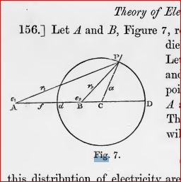
MAX-fig-8.JPG
100%
17.17 KB complete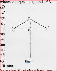
maxwell figure 9 "A TREATISE ON ELECTRICITY AND MAGNETISM"
MAX-fig-10.JPG
100%
22.63 KB complete
MAX-fig-11.JPG
100%
19.25 KB complete
MAX-fig-12.JPG
100%
19.81 KB complete
MAX-fig-13.JPG
100%
27.50 KB complete
MAX-fig-14.JPG
100%
21.26 KB complete
MAX-fig-16.JPG
100%
23.60 KB complete
MAX-fig-17-ver2.JPG
100%
15.62 KB complete
MAX-fig-17.JPG
100%
29.45 KB complete
MAX-fig-18.JPG
100%
31.91 KB complete
MAX-fig-19.JPG
100%
21.35 KB complete
MAX-fig-21.JPG
100%
33.02 KB complete
MAX-fig-25.JPG
100%
25.91 KB complete
MAX-fig-27.JPG
100%
30.88 KB complete
MAX-fig-28.JPG
100%
30.38 KB complete
MAX-fig-28.JPG
100%
30.38 KB complete
MAX-fig-29.JPG
100%
22.12 KB complete
MAX-fig-32.JPG
100%
31.58 KB complete
MAX-fig-35.JPG
100%
39.50 KB complete
MAX-fig-36.JPG
100%
27.75 KB complete
MAX-fig-37.JPG
100%
28.10 KB complete
MAX-fig-38.JPG
100%
21.80 KB complete
MAX-fig-60.JPG
100%
152.98 KB complete
MAX-fig-61.JPG
100%
159.54 KB complete
MAX-fig-63.JPG
100%
142.14 KB complete
MAX-fig-64.JPG
100%
149.13 KB complete
SOURCE: https://en.wikipedia.org/wiki/Maxwell%27s_equations
h
https://en.wikipedia.org/wiki/Maxwell%27s_equations
AAAAAAAAAAAAAAAAAAAAAAAAAAAAAAAAAAAAAAAA
Maxwell's equations
From Wikipedia, the free encyclopedia ( Jump to navigationJump to search )
For thermodynamic relations, see Maxwell relations.
For the history of the equations, see History of Maxwell's equations.
For a general description of electromagnetism, see Electromagnetism.
Articles about
Electromagnetism
Solenoid
ElectricityMagnetismHistoryTextbooks
Electrostatics
Magnetostatics
Electrodynamics
Lorentz force lawElectromagnetic inductionFaraday's lawLenz's lawDisplacement currentMagnetic vector potentialMaxwell's equationsElectromagnetic fieldElectromagnetic pulseElectromagnetic radiationMaxwell tensorPoynting vectorLiénard–Wiechert potentialJefimenko's equationsEddy currentLondon equations
Mathematical descriptions of the electromagnetic field
Electrical network
Covariant formulation
Scientists
CCCCCCCCCCCCCCCCCCCCCCCCCCCCCCCCCCC
Maxwell's equations are a set of coupled partial differential equations that, together with the Lorentz force law, form the foundation of classical electromagnetism, classical optics, and electric circuits. The equations provide a mathematical model for electric, optical, and radio technologies, such as power generation, electric motors, wireless communication, lenses, radar etc. They describe how electric and magnetic fields are generated by charges, currents, and changes of the fields.[note 1] The equations are named after the physicist and mathematician James Clerk Maxwell, who, in 1861 and 1862, published an early form of the equations that included the Lorentz force law. Maxwell first used the equations to propose that light is an electromagnetic phenomenon.
An important consequence of Maxwell's equations is that they demonstrate how fluctuating electric and magnetic fields propagate at a constant speed (c) in a vacuum. Known as electromagnetic radiation, these waves may occur at various wavelengths to produce a spectrum of light from radio waves to gamma rays.
The equations have two major variants. The microscopic equations have universal applicability but are unwieldy for common calculations. They relate the electric and magnetic fields to total charge and total current, including the complicated charges and currents in materials at the atomic scale. The macroscopic equations define two new auxiliary fields that describe the large-scale behaviour of matter without having to consider atomic scale charges and quantum phenomena like spins. However, their use requires experimentally determined parameters for a phenomenological description of the electromagnetic response of materials.
The term "Maxwell's equations" is often also used for equivalent alternative formulations. Versions of Maxwell's equations based on the electric and magnetic scalar potentials are preferred for explicitly solving the equations as a boundary value problem, analytical mechanics, or for use in quantum mechanics. The covariant formulation (on spacetime rather than space and time separately) makes the compatibility of Maxwell's equations with special relativity manifest. Maxwell's equations in curved spacetime, commonly used in high energy and gravitational physics, are compatible with general relativity.[note 2] In fact, Albert Einstein developed special and general relativity to accommodate the invariant speed of light, a consequence of Maxwell's equations, with the principle that only relative movement has physical consequences.
The publication of the equations marked the unification of a theory for previously separately described phenomena: magnetism, electricity, light and associated radiation. Since the mid-20th century, it has been understood that Maxwell's equations do not give an exact description of electromagnetic phenomena, but are instead a classical limit of the more precise theory of quantum electrodynamics.
Contents
1 Conceptual descriptions
1.1 Gauss's law
1.2 Gauss's law for magnetism
1.3 Faraday's law
1.4 Ampère's law with Maxwell's addition
2 Formulation in terms of electric and magnetic fields (microscopic or in vacuum version)
2.1 Key to the notation
2.1.1 Differential equations
2.1.2 Integral equations
2.2 Formulation in SI units convention
2.3 Formulation in Gaussian units convention
3 Relationship between differential and integral formulations
3.1 Flux and divergence
3.2 Circulation and curl
4 Charge conservation
5 Vacuum equations, electromagnetic waves and speed of light
6 Macroscopic formulation
6.1 Bound charge and current
6.2 Auxiliary fields, polarization and magnetization
6.3 Constitutive relations
7 Alternative formulations
8 Relativistic formulations
9 Solutions
10 Overdetermination of Maxwell's equations
11 Maxwell's equations as the classical limit of QED
12 Variations
12.1 Magnetic monopoles
13 See also
14 Notes
15 References
16 Historical publications
17 Further reading
18 External links
18.1 Modern treatments
18.2 Other
Conceptual descriptions
Gauss's law
Main article: Gauss's law
Gauss's law describes the relationship between a static electric field and the electric charges that cause it: a static electric field points away from positive charges and towards negative charges, and the net outflow of the electric field through any closed surface is proportional to the charge enclosed by the surface. This means that the net flux passing through a closed surface yields the total charge (including bound charge due to polarization of material) enclosed by that surface, divided by dielectricity of free space (the vacuum permittivity).
Gauss's law for magnetism: magnetic field lines never begin nor end but form loops or extend to infinity as shown here with the magnetic field due to a ring of current.
Gauss's law for magnetism
Main article: Gauss's law for magnetism
Gauss's law for magnetism states that there are no "magnetic charges" (also called magnetic monopoles), analogous to electric charges.[1] Instead, the magnetic field due to materials is generated by a configuration called a dipole, and the net outflow of the magnetic field through any closed surface is zero. Magnetic dipoles are best represented as loops of current but resemble positive and negative 'magnetic charges', inseparably bound together, having no net 'magnetic charge'. Equivalent technical statements are that the sum total magnetic flux through any Gaussian surface is zero, or that the magnetic field is a solenoidal vector field.[note 3]
Faraday's law
Main article: Faraday's law of induction
In a geomagnetic storm, a surge in the flux of charged particles temporarily alters Earth's magnetic field, which induces electric fields in Earth's atmosphere, thus causing surges in electrical power grids. (Not to scale.)
The Maxwell–Faraday version of Faraday's law of induction describes how a time varying magnetic field creates ("induces") an electric field.[1] In integral form, it states that the work per unit charge required to move a charge around a closed loop equals the rate of change of the magnetic flux through the enclosed surface.
The electromagnetic induction is the operating principle behind many electric generators: for example, a rotating bar magnet creates a changing magnetic field, which in turn generates an electric field in a nearby wire.
Ampère's law with Maxwell's addition
Main article: Ampère's circuital law
Magnetic core memory (1954) is an application of Ampère's law. Each core stores one bit of data.
Ampère's law with Maxwell's addition states that magnetic fields can be generated in two ways: by electric current (this was the original "Ampère's law") and by changing electric fields (this was "Maxwell's addition", which he called displacement current). In integral form, the magnetic field induced around any closed loop is proportional to the electric current plus displacement current (proportional to the rate of change of electric flux) through the enclosed surface.
Maxwell's addition to Ampère's law is particularly important: it makes the set of equations mathematically consistent for non static fields, without changing the laws of Ampere and Gauss for static fields.[2] However, as a consequence, it predicts that a changing magnetic field induces an electric field and vice versa.[1][3] Therefore, these equations allow self-sustaining "electromagnetic waves" to travel through empty space (see electromagnetic wave equation).
The speed calculated for electromagnetic waves, which could be predicted from experiments on charges and currents,[note 4] matches the speed of light; indeed, light is one form of electromagnetic radiation (as are X-rays, radio waves, and others). Maxwell understood the connection between electromagnetic waves and light in 1861, thereby unifying the theories of electromagnetism and optics.
Formulation in terms of electric and magnetic fields (microscopic or in vacuum version)
In the electric and magnetic field formulation there are four equations that determine the fields for given charge and current distribution. A separate law of nature, the Lorentz force law, describes how, conversely, the electric and magnetic fields act on charged particles and currents. A version of this law was included in the original equations by Maxwell but, by convention, is included no longer. The vector calculus formalism below, the work of Oliver Heaviside,[4][5] has become standard. It is manifestly rotation invariant, and therefore mathematically much more transparent than Maxwell's original 20 equations in x,y,z components. The relativistic formulations are even more symmetric and manifestly Lorentz invariant. For the same equations expressed using tensor calculus or differential forms, see alternative formulations.
The differential and integral formulations are mathematically equivalent and are both useful. The integral formulation relates fields within a region of space to fields on the boundary and can often be used to simplify and directly calculate fields from symmetric distributions of charges and currents. On the other hand, the differential equations are purely local and are a more natural starting point for calculating the fields in more complicated (less symmetric) situations, for example using finite element analysis.[6]
Key to the notation
Symbols in bold represent vector quantities, and symbols in italics represent scalar quantities, unless otherwise indicated. The equations introduce the electric field, E, a vector field, and the magnetic field, B, a pseudovector field, each generally having a time and location dependence. The sources are
the total electric charge density (total charge per unit volume), ρ, and
the total electric current density (total current per unit area), J.
The universal constants appearing in the equations (the first two ones explicitly only in the SI units formulation) are:
the permittivity of free space, ε0, and
the permeability of free space, μ0, and
the speed of light, {\displaystyle c={\frac {1}{\sqrt {\varepsilon _{0}\mu _{0}}}}}{\displaystyle c={\frac {1}{\sqrt {\varepsilon _{0}\mu _{0}}}}}
Differential equations
In the differential equations,
the nabla symbol, ∇, denotes the three-dimensional gradient operator, del,
the ∇⋅ symbol (pronounced "del dot") denotes the divergence operator,
the ∇× symbol (pronounced "del cross") denotes the curl operator.
Integral equations
In the integral equations,
Ω is any fixed volume with closed boundary surface ∂Ω, and
Σ is any fixed surface with closed boundary curve ∂Σ,
Here a fixed volume or surface means that it does not change over time. The equations are correct, complete, and a little easier to interpret with time-independent surfaces. For example, since the surface is time-independent, we can bring the differentiation under the integral sign in Faraday's law:
{\displaystyle {\frac {d}{dt}}\iint _{\Sigma }\mathbf {B} \cdot \mathrm {d} \mathbf {S} =\iint _{\Sigma }{\frac {\partial \mathbf {B} }{\partial t}}\cdot \mathrm {d} \mathbf {S} \,,}{\frac {d}{dt}}\iint _{\Sigma }\mathbf {B} \cdot \mathrm {d} \mathbf {S} =\iint _{\Sigma }{\frac {\partial \mathbf {B} }{\partial t}}\cdot \mathrm {d} \mathbf {S} \,,
Maxwell's equations can be formulated with possibly time-dependent surfaces and volumes by using the differential version and using Gauss and Stokes formula appropriately.
\oiint{\displaystyle {\scriptstyle \partial \Omega }}{\scriptstyle \partial \Omega } is a surface integral over the boundary surface ∂Ω, with the loop indicating the surface is closed
{\displaystyle \iiint _{\Omega }}\iiint _{\Omega } is a volume integral over the volume Ω,
{\displaystyle \oint _{\partial \Sigma }}\oint _{\partial \Sigma } is a line integral around the boundary curve ∂Σ, with the loop indicating the curve is closed.
{\displaystyle \iint _{\Sigma }}\iint _{\Sigma } is a surface integral over the surface Σ,
The total electric charge Q enclosed in Ω is the volume integral over Ω of the charge density ρ (see the "macroscopic formulation" section below):
{\displaystyle Q=\iiint _{\Omega }\rho \ \mathrm {d} V,}{\displaystyle Q=\iiint _{\Omega }\rho \ \mathrm {d} V,}
where dV is the volume element.
The net electric current I is the surface integral of the electric current density J passing through a fixed surface, Σ:
{\displaystyle I=\iint _{\Sigma }\mathbf {J} \cdot \mathrm {d} \mathbf {S} ,}{\displaystyle I=\iint _{\Sigma }\mathbf {J} \cdot \mathrm {d} \mathbf {S} ,}
where dS denotes the differential vector element of surface area S, normal to surface Σ. (Vector area is sometimes denoted by A rather than S, but this conflicts with the notation for magnetic vector potential).
Formulation in SI units convention
Name Integral equations Differential equations
Gauss's law \oiint{\displaystyle {\scriptstyle \partial \Omega }}{\scriptstyle \partial \Omega } {\displaystyle \mathbf {E} \cdot \mathrm {d} \mathbf {S} ={\frac {1}{\varepsilon _{0}}}\iiint _{\Omega }\rho \,\mathrm {d} V}\mathbf {E} \cdot \mathrm {d} \mathbf {S} ={\frac {1}{\varepsilon _{0}}}\iiint _{\Omega }\rho \,\mathrm {d} V {\displaystyle \nabla \cdot \mathbf {E} ={\frac {\rho }{\varepsilon _{0}}}}\nabla \cdot \mathbf {E} ={\frac {\rho }{\varepsilon _{0}}}
Gauss's law for magnetism \oiint{\displaystyle {\scriptstyle \partial \Omega }}{\scriptstyle \partial \Omega } {\displaystyle \mathbf {B} \cdot \mathrm {d} \mathbf {S} =0}\mathbf {B} \cdot \mathrm {d} \mathbf {S} =0 {\displaystyle \nabla \cdot \mathbf {B} =0}\nabla \cdot \mathbf {B} =0
Maxwell–Faraday equation
(Faraday's law of induction)
{\displaystyle \oint _{\partial \Sigma }\mathbf {E} \cdot \mathrm {d} {\boldsymbol {\ell }}=-{\frac {\mathrm {d} }{\mathrm {d} t}}\iint _{\Sigma }\mathbf {B} \cdot \mathrm {d} \mathbf {S} }\oint _{\partial \Sigma }\mathbf {E} \cdot \mathrm {d} {\boldsymbol {\ell }}=-{\frac {\mathrm {d} }{\mathrm {d} t}}\iint _{\Sigma }\mathbf {B} \cdot \mathrm {d} \mathbf {S} {\displaystyle \nabla \times \mathbf {E} =-{\frac {\partial \mathbf {B} }{\partial t}}}\nabla \times \mathbf {E} =-{\frac {\partial \mathbf {B} }{\partial t}}
Ampère's circuital law (with Maxwell's addition) {\displaystyle {\begin{aligned}\oint _{\partial \Sigma }&\mathbf {B} \cdot \mathrm {d} {\boldsymbol {\ell }}=\mu _{0}\left(\iint _{\Sigma }\mathbf {J} \cdot \mathrm {d} \mathbf {S} +\varepsilon _{0}{\frac {\mathrm {d} }{\mathrm {d} t}}\iint _{\Sigma }\mathbf {E} \cdot \mathrm {d} \mathbf {S} \right)\\\end{aligned}}}{\displaystyle {\begin{aligned}\oint _{\partial \Sigma }&\mathbf {B} \cdot \mathrm {d} {\boldsymbol {\ell }}=\mu _{0}\left(\iint _{\Sigma }\mathbf {J} \cdot \mathrm {d} \mathbf {S} +\varepsilon _{0}{\frac {\mathrm {d} }{\mathrm {d} t}}\iint _{\Sigma }\mathbf {E} \cdot \mathrm {d} \mathbf {S} \right)\\\end{aligned}}} {\displaystyle \nabla \times \mathbf {B} =\mu _{0}\left(\mathbf {J} +\varepsilon _{0}{\frac {\partial \mathbf {E} }{\partial t}}\right)}\nabla \times \mathbf {B} =\mu _{0}\left(\mathbf {J} +\varepsilon _{0}{\frac {\partial \mathbf {E} }{\partial t}}\right)
Formulation in Gaussian units convention
Main article: Gaussian units
The definitions of charge, electric field, and magnetic field can be altered to simplify theoretical calculation, by absorbing dimensioned factors of ε0 and μ0 into the units of calculation, by convention. With a corresponding change in convention for the Lorentz force law this yields the same physics, i.e. trajectories of charged particles, or work done by an electric motor. These definitions are often preferred in theoretical and high energy physics where it is natural to take the electric and magnetic field with the same units, to simplify the appearance of the electromagnetic tensor: the Lorentz covariant object unifying electric and magnetic field would then contain components with uniform unit and dimension.[7]:vii Such modified definitions are conventionally used with the Gaussian (CGS) units. Using these definitions and conventions, colloquially "in Gaussian units",[8] the Maxwell equations become:[9]
Name Integral equations Differential equations
Gauss's law \oiint{\displaystyle {\scriptstyle \partial \Omega }}{\scriptstyle \partial \Omega } {\displaystyle \mathbf {E} \cdot \mathrm {d} \mathbf {S} =4\pi \iiint _{\Omega }\rho \,\mathrm {d} V}{\displaystyle \mathbf {E} \cdot \mathrm {d} \mathbf {S} =4\pi \iiint _{\Omega }\rho \,\mathrm {d} V} {\displaystyle \nabla \cdot \mathbf {E} =4\pi \rho }\nabla \cdot \mathbf {E} =4\pi \rho
Gauss's law for magnetism \oiint{\displaystyle {\scriptstyle \partial \Omega }}{\scriptstyle \partial \Omega } {\displaystyle \mathbf {B} \cdot \mathrm {d} \mathbf {S} =0}\mathbf {B} \cdot \mathrm {d} \mathbf {S} =0 {\displaystyle \nabla \cdot \mathbf {B} =0}\nabla \cdot \mathbf {B} =0
Maxwell–Faraday equation
(Faraday's law of induction)
{\displaystyle \oint _{\partial \Sigma }\mathbf {E} \cdot \mathrm {d} {\boldsymbol {\ell }}=-{\frac {1}{c}}{\frac {\mathrm {d} }{\mathrm {d} t}}\iint _{\Sigma }\mathbf {B} \cdot \mathrm {d} \mathbf {S} }{\displaystyle \oint _{\partial \Sigma }\mathbf {E} \cdot \mathrm {d} {\boldsymbol {\ell }}=-{\frac {1}{c}}{\frac {\mathrm {d} }{\mathrm {d} t}}\iint _{\Sigma }\mathbf {B} \cdot \mathrm {d} \mathbf {S} } {\displaystyle \nabla \times \mathbf {E} =-{\frac {1}{c}}{\frac {\partial \mathbf {B} }{\partial t}}}\nabla \times \mathbf {E} =-{\frac {1}{c}}{\frac {\partial \mathbf {B} }{\partial t}}
Ampère's circuital law (with Maxwell's addition) {\displaystyle {\begin{aligned}\oint _{\partial \Sigma }&\mathbf {B} \cdot \mathrm {d} {\boldsymbol {\ell }}={\frac {1}{c}}\left(4\pi \iint _{\Sigma }\mathbf {J} \cdot \mathrm {d} \mathbf {S} +{\frac {\mathrel {\mathrm {d} }}{\mathrm {d} t}}\iint _{\Sigma }\mathbf {E} \cdot \mathrm {d} \mathbf {S} \right)\end{aligned}}}{\displaystyle {\begin{aligned}\oint _{\partial \Sigma }&\mathbf {B} \cdot \mathrm {d} {\boldsymbol {\ell }}={\frac {1}{c}}\left(4\pi \iint _{\Sigma }\mathbf {J} \cdot \mathrm {d} \mathbf {S} +{\frac {\mathrel {\mathrm {d} }}{\mathrm {d} t}}\iint _{\Sigma }\mathbf {E} \cdot \mathrm {d} \mathbf {S} \right)\end{aligned}}} {\displaystyle \nabla \times \mathbf {B} ={\frac {1}{c}}\left(4\pi \mathbf {J} +{\frac {\partial \mathbf {E} }{\partial t}}\right)}{\displaystyle \nabla \times \mathbf {B} ={\frac {1}{c}}\left(4\pi \mathbf {J} +{\frac {\partial \mathbf {E} }{\partial t}}\right)}
The equations are particularly readable when length and time are measured in compatible units like seconds and lightseconds i.e. in units such that c = 1 unit of length/unit of time. Ever since 1983 (see International System of Units), metres and seconds are compatible except for historical legacy since by definition c = 299 792 458 m/s (≈ 1.0 feet/nanosecond).
Further cosmetic changes, called rationalisations, are possible by absorbing factors of 4π depending on whether we want Coulomb's law or Gauss's law to come out nicely, see Lorentz-Heaviside units (used mainly in particle physics). In theoretical physics it is often useful to choose units such that Planck's constant, the elementary charge, and even Newton's constant are 1. See Planck units.
Relationship between differential and integral formulations
The equivalence of the differential and integral formulations are a consequence of the Gauss divergence theorem and the Kelvin–Stokes theorem.
Flux and divergence
Volume Ω and its closed boundary ∂Ω, containing (respectively enclosing) a source (+) and sink (−) of a vector field F. Here, F could be the E field with source electric charges, but not the B field, which has no magnetic charges as shown. The outward unit normal is n.
According to the (purely mathematical) Gauss divergence theorem, the electric flux through the boundary surface ∂Ω can be rewritten as
\oiint{\displaystyle {\scriptstyle \partial \Omega }}{\scriptstyle \partial \Omega } {\displaystyle \mathbf {E} \cdot \mathrm {d} \mathbf {S} =\iiint _{\Omega }\nabla \cdot \mathbf {E} \,\mathrm {d} V}{\displaystyle \mathbf {E} \cdot \mathrm {d} \mathbf {S} =\iiint _{\Omega }\nabla \cdot \mathbf {E} \,\mathrm {d} V}
The integral version of Gauss's equation can thus be rewritten as
{\displaystyle \iiint _{\Omega }\left(\nabla \cdot \mathbf {E} -{\frac {\rho }{\varepsilon _{0}}}\right)\,\mathrm {d} V=0}{\displaystyle \iiint _{\Omega }\left(\nabla \cdot \mathbf {E} -{\frac {\rho }{\varepsilon _{0}}}\right)\,\mathrm {d} V=0}
Since Ω is arbitrary (e.g. an arbitrary small ball with arbitrary center), this is satisfied if and only if the integrand is zero everywhere. This is the differential equations formulation of Gauss equation up to a trivial rearrangement.
Similarly rewriting the magnetic flux in Gauss's law for magnetism in integral form gives
\oiint{\displaystyle {\scriptstyle \partial \Omega }}{\scriptstyle \partial \Omega } {\displaystyle \mathbf {B} \cdot \mathrm {d} \mathbf {S} =\iiint _{\Omega }\nabla \cdot \mathbf {B} \,\mathrm {d} V=0}{\displaystyle \mathbf {B} \cdot \mathrm {d} \mathbf {S} =\iiint _{\Omega }\nabla \cdot \mathbf {B} \,\mathrm {d} V=0}.
which is satisfied for all Ω if and only if {\displaystyle \nabla \cdot \mathbf {B} =0}\nabla \cdot {\mathbf {B}}=0 everywhere.
Circulation and curl
Surface Σ with closed boundary ∂Σ. F could be the E or B fields. Again, n is the unit normal. (The curl of a vector field doesn't literally look like the "circulations", this is a heuristic depiction.)
By the Kelvin–Stokes theorem we can rewrite the line integrals of the fields around the closed boundary curve ∂Σ to an integral of the "circulation of the fields" (i.e. their curls) over a surface it bounds, i.e.
{\displaystyle \oint _{\partial \Sigma }\mathbf {B} \cdot \mathrm {d} {\boldsymbol {\ell }}=\iint _{\Sigma }(\nabla \times \mathbf {B} )\cdot \mathrm {d} \mathbf {S} }{\displaystyle \oint _{\partial \Sigma }\mathbf {B} \cdot \mathrm {d} {\boldsymbol {\ell }}=\iint _{\Sigma }(\nabla \times \mathbf {B} )\cdot \mathrm {d} \mathbf {S} },
Hence the modified Ampere law in integral form can be rewritten as
{\displaystyle \iint _{\Sigma }\left(\nabla \times \mathbf {B} -\mu _{0}\left(\mathbf {J} +\varepsilon _{0}{\frac {\partial \mathbf {E} }{\partial t}}\right)\right)\cdot \mathrm {d} \mathbf {S} =0}{\displaystyle \iint _{\Sigma }\left(\nabla \times \mathbf {B} -\mu _{0}\left(\mathbf {J} +\varepsilon _{0}{\frac {\partial \mathbf {E} }{\partial t}}\right)\right)\cdot \mathrm {d} \mathbf {S} =0}.
Since Σ can be chosen arbitrarily, e.g. as an arbitrary small, arbitrary oriented, and arbitrary centered disk, we conclude that the integrand is zero iff Ampere's modified law in differential equations form is satisfied. The equivalence of Faraday's law in differential and integral form follows likewise.
The line integrals and curls are analogous to quantities in classical fluid dynamics: the circulation of a fluid is the line integral of the fluid's flow velocity field around a closed loop, and the vorticity of the fluid is the curl of the velocity field.
Charge conservation
The invariance of charge can be derived as a corollary of Maxwell's equations. The left-hand side of the modified Ampere's Law has zero divergence by the div–curl identity. Expanding the divergence of the right-hand side, interchanging derivatives, and applying Gauss's law gives:
{\displaystyle 0=\nabla \cdot \nabla \times \mathbf {B} =\mu _{0}\left(\nabla \cdot \mathbf {J} +\varepsilon _{0}{\frac {\partial }{\partial t}}\nabla \cdot \mathbf {E} \right)=\mu _{0}\left(\nabla \cdot \mathbf {J} +{\frac {\partial \rho }{\partial t}}\right)}{\displaystyle 0=\nabla \cdot \nabla \times \mathbf {B} =\mu _{0}\left(\nabla \cdot \mathbf {J} +\varepsilon _{0}{\frac {\partial }{\partial t}}\nabla \cdot \mathbf {E} \right)=\mu _{0}\left(\nabla \cdot \mathbf {J} +{\frac {\partial \rho }{\partial t}}\right)}
i.e.
{\displaystyle {\frac {\partial \rho }{\partial t}}+\nabla \cdot \mathbf {J} =0}{\displaystyle {\frac {\partial \rho }{\partial t}}+\nabla \cdot \mathbf {J} =0}.
By the Gauss Divergence Theorem, this means the rate of change of charge in a fixed volume equals the net current flowing through the boundary:
{\displaystyle {\frac {d}{dt}}Q_{\Omega }={\frac {d}{dt}}\iiint _{\Omega }\rho \mathrm {d} V=-}{\displaystyle {\frac {d}{dt}}Q_{\Omega }={\frac {d}{dt}}\iiint _{\Omega }\rho \mathrm {d} V=-} \oiint{\displaystyle {\scriptstyle \partial \Omega }}{\scriptstyle \partial \Omega } {\displaystyle \mathbf {J} \cdot {\rm {d}}\mathbf {S} =-I_{\partial \Omega }.}{\displaystyle \mathbf {J} \cdot {\rm {d}}\mathbf {S} =-I_{\partial \Omega }.}
In particular, in an isolated system the total charge is conserved.
Vacuum equations, electromagnetic waves and speed of light
Further information: Electromagnetic wave equation, Inhomogeneous electromagnetic wave equation, Sinusoidal plane-wave solutions of the electromagnetic wave equation, and Helmholtz equation
This 3D diagram shows a plane linearly polarized wave propagating from left to right, defined by E = E0 sin(−ωt + k ⋅ r) and B = B0 sin(−ωt + k ⋅ r) The oscillating fields are detected at the flashing point. The horizontal wavelength is λ. E0 ⋅ B0 = 0 = E0 ⋅ k = B0 ⋅ k
In a region with no charges (ρ = 0) and no currents (J = 0), such as in a vacuum, Maxwell's equations reduce to:
{\displaystyle {\begin{aligned}\nabla \cdot \mathbf {E} &=0\quad &\nabla \times \mathbf {E} &=-{\frac {\partial \mathbf {B} }{\partial t}},\\\nabla \cdot \mathbf {B} &=0\quad &\nabla \times \mathbf {B} &=\mu _{0}\varepsilon _{0}{\frac {\partial \mathbf {E} }{\partial t}}.\end{aligned}}}{\displaystyle {\begin{aligned}\nabla \cdot \mathbf {E} &=0\quad &\nabla \times \mathbf {E} &=-{\frac {\partial \mathbf {B} }{\partial t}},\\\nabla \cdot \mathbf {B} &=0\quad &\nabla \times \mathbf {B} &=\mu _{0}\varepsilon _{0}{\frac {\partial \mathbf {E} }{\partial t}}.\end{aligned}}}
Taking the curl (∇×) of the curl equations, and using the curl of the curl identity we obtain
{\displaystyle {\begin{aligned}\mu _{0}\varepsilon _{0}{\frac {\partial ^{2}\mathbf {E} }{\partial t^{2}}}-\nabla ^{2}\mathbf {E} =0\\\mu _{0}\varepsilon _{0}{\frac {\partial ^{2}\mathbf {B} }{\partial t^{2}}}-\nabla ^{2}\mathbf {B} =0\end{aligned}}}{\displaystyle {\begin{aligned}\mu _{0}\varepsilon _{0}{\frac {\partial ^{2}\mathbf {E} }{\partial t^{2}}}-\nabla ^{2}\mathbf {E} =0\\\mu _{0}\varepsilon _{0}{\frac {\partial ^{2}\mathbf {B} }{\partial t^{2}}}-\nabla ^{2}\mathbf {B} =0\end{aligned}}}
The quantity {\displaystyle \mu _{0}\varepsilon _{0}}{\displaystyle \mu _{0}\varepsilon _{0}} has the dimension of (time/length)2. Defining {\displaystyle c=(\mu _{0}\varepsilon _{0})^{-1/2}}{\displaystyle c=(\mu _{0}\varepsilon _{0})^{-1/2}}, the equations above have the form of the standard wave equations
{\displaystyle {\begin{aligned}{\frac {1}{c^{2}}}{\frac {\partial ^{2}\mathbf {E} }{\partial t^{2}}}-\nabla ^{2}\mathbf {E} =0\\{\frac {1}{c^{2}}}{\frac {\partial ^{2}\mathbf {B} }{\partial t^{2}}}-\nabla ^{2}\mathbf {B} =0\end{aligned}}}{\displaystyle {\begin{aligned}{\frac {1}{c^{2}}}{\frac {\partial ^{2}\mathbf {E} }{\partial t^{2}}}-\nabla ^{2}\mathbf {E} =0\\{\frac {1}{c^{2}}}{\frac {\partial ^{2}\mathbf {B} }{\partial t^{2}}}-\nabla ^{2}\mathbf {B} =0\end{aligned}}}
Already during Maxwell's lifetime, it was found that the known values for {\displaystyle \varepsilon _{0}}\varepsilon _{0} and {\displaystyle \mu _{0}}\mu _{0} give {\displaystyle c\approx 2.998\times 10^{8}\,{\text{m/s}}}{\displaystyle c\approx 2.998\times 10^{8}\,{\text{m/s}}}, then already known to be the speed of light in free space. This led him to propose that light and radio waves were propagating electromagnetic waves, since amply confirmed. In the old SI system of units, the values of {\displaystyle \mu _{0}=4\pi \times 10^{-7}}{\displaystyle \mu _{0}=4\pi \times 10^{-7}} and {\displaystyle c=299792458\,{\text{m/s}}}{\displaystyle c=299792458\,{\text{m/s}}} are defined constants, (which means that by definition {\displaystyle \varepsilon _{0}=8.854...\times 10^{-12}\,{\text{F/m}}}{\displaystyle \varepsilon _{0}=8.854...\times 10^{-12}\,{\text{F/m}}}) that define the ampere and the metre. In the new SI system, only c keeps its defined value, and the electron charge gets a defined value.
In materials with relative permittivity, εr, and relative permeability, μr, the phase velocity of light becomes
{\displaystyle v_{\text{p}}={\frac {1}{\sqrt {\mu _{0}\mu _{\text{r}}\varepsilon _{0}\varepsilon _{\text{r}}}}}}v_{\text{p}}={\frac {1}{\sqrt {\mu _{0}\mu _{\text{r}}\varepsilon _{0}\varepsilon _{\text{r}}}}}
which is usually[note 5] less than c.
In addition, E and B are perpendicular to each other and to the direction of wave propagation, and are in phase with each other. A sinusoidal plane wave is one special solution of these equations. Maxwell's equations explain how these waves can physically propagate through space. The changing magnetic field creates a changing electric field through Faraday's law. In turn, that electric field creates a changing magnetic field through Maxwell's addition to Ampère's law. This perpetual cycle allows these waves, now known as electromagnetic radiation, to move through space at velocity c.
Macroscopic formulation
The above equations are the microscopic version of Maxwell's equations, expressing the electric and the magnetic fields in terms of the (possibly atomic-level) charges and currents present. This is sometimes called the "general" form, but the macroscopic version below is equally general, the difference being one of bookkeeping.
The microscopic version is sometimes called "Maxwell's equations in a vacuum": this refers to the fact that the material medium is not built into the structure of the equations, but appears only in the charge and current terms. The microscopic version was introduced by Lorentz, who tried to use it to derive the macroscopic properties of bulk matter from its microscopic constituents.[10]:5
"Maxwell's macroscopic equations", also known as Maxwell's equations in matter, are more similar to those that Maxwell introduced himself.
Name Integral equations (SI convention) Differential equations (SI convention) Differential equations (Gaussian convention)
Gauss's law \oiint{\displaystyle {\scriptstyle \partial \Omega }}{\scriptstyle \partial \Omega } {\displaystyle \mathbf {D} \cdot \mathrm {d} \mathbf {S} =\iiint _{\Omega }\rho _{\text{f}}\,\mathrm {d} V}\mathbf {D} \cdot \mathrm {d} \mathbf {S} =\iiint _{\Omega }\rho _{\text{f}}\,\mathrm {d} V {\displaystyle \nabla \cdot \mathbf {D} =\rho _{\text{f}}}\nabla \cdot \mathbf {D} =\rho _{\text{f}} {\displaystyle \nabla \cdot \mathbf {D} =4\pi \rho _{\text{f}}}\nabla \cdot \mathbf {D} =4\pi \rho _{\text{f}}
Gauss's law for magnetism \oiint{\displaystyle {\scriptstyle \partial \Omega }}{\scriptstyle \partial \Omega } {\displaystyle \mathbf {B} \cdot \mathrm {d} \mathbf {S} =0}\mathbf {B} \cdot \mathrm {d} \mathbf {S} =0 {\displaystyle \nabla \cdot \mathbf {B} =0}\nabla \cdot \mathbf {B} =0 {\displaystyle \nabla \cdot \mathbf {B} =0}\nabla \cdot \mathbf {B} =0
Maxwell–Faraday equation (Faraday's law of induction) {\displaystyle \oint _{\partial \Sigma }\mathbf {E} \cdot \mathrm {d} {\boldsymbol {\ell }}=-{\frac {d}{dt}}\iint _{\Sigma }\mathbf {B} \cdot \mathrm {d} \mathbf {S} }\oint _{\partial \Sigma }\mathbf {E} \cdot \mathrm {d} {\boldsymbol {\ell }}=-{\frac {d}{dt}}\iint _{\Sigma }\mathbf {B} \cdot \mathrm {d} \mathbf {S} {\displaystyle \nabla \times \mathbf {E} =-{\frac {\partial \mathbf {B} }{\partial t}}}\nabla \times \mathbf {E} =-{\frac {\partial \mathbf {B} }{\partial t}} {\displaystyle \nabla \times \mathbf {E} =-{\frac {1}{c}}{\frac {\partial \mathbf {B} }{\partial t}}}\nabla \times \mathbf {E} =-{\frac {1}{c}}{\frac {\partial \mathbf {B} }{\partial t}}
Ampère's circuital law (with Maxwell's addition) {\displaystyle {\begin{aligned}\oint _{\partial \Sigma }&\mathbf {H} \cdot \mathrm {d} {\boldsymbol {\ell }}=\\&\iint _{\Sigma }\mathbf {J} _{\text{f}}\cdot \mathrm {d} \mathbf {S} +{\frac {d}{dt}}\iint _{\Sigma }\mathbf {D} \cdot \mathrm {d} \mathbf {S} \\\end{aligned}}}{\displaystyle {\begin{aligned}\oint _{\partial \Sigma }&\mathbf {H} \cdot \mathrm {d} {\boldsymbol {\ell }}=\\&\iint _{\Sigma }\mathbf {J} _{\text{f}}\cdot \mathrm {d} \mathbf {S} +{\frac {d}{dt}}\iint _{\Sigma }\mathbf {D} \cdot \mathrm {d} \mathbf {S} \\\end{aligned}}} {\displaystyle \nabla \times \mathbf {H} =\mathbf {J} _{\text{f}}+{\frac {\partial \mathbf {D} }{\partial t}}}\nabla \times \mathbf {H} =\mathbf {J} _{\text{f}}+{\frac {\partial \mathbf {D} }{\partial t}} {\displaystyle \nabla \times \mathbf {H} ={\frac {1}{c}}\left(4\pi \mathbf {J} _{\text{f}}+{\frac {\partial \mathbf {D} }{\partial t}}\right)}\nabla \times \mathbf {H} ={\frac {1}{c}}\left(4\pi \mathbf {J} _{\text{f}}+{\frac {\partial \mathbf {D} }{\partial t}}\right)
In the macroscopic equations, the influence of bound charge Qb and bound current Ib is incorporated into the displacement field D and the magnetizing field H, while the equations depend only on the free charges Qf and free currents If. This reflects a splitting of the total electric charge Q and current I (and their densities ρ and J) into free and bound parts:
{\displaystyle {\begin{aligned}Q&=Q_{\text{f}}+Q_{\text{b}}=\iiint _{\Omega }\left(\rho _{\text{f}}+\rho _{\text{b}}\right)\,\mathrm {d} V=\iiint _{\Omega }\rho \,\mathrm {d} V\\I&=I_{\text{f}}+I_{\text{b}}=\iint _{\Sigma }\left(\mathbf {J} _{\text{f}}+\mathbf {J} _{\text{b}}\right)\cdot \mathrm {d} \mathbf {S} =\iint _{\Sigma }\mathbf {J} \cdot \mathrm {d} \mathbf {S} \end{aligned}}}{\displaystyle {\begin{aligned}Q&=Q_{\text{f}}+Q_{\text{b}}=\iiint _{\Omega }\left(\rho _{\text{f}}+\rho _{\text{b}}\right)\,\mathrm {d} V=\iiint _{\Omega }\rho \,\mathrm {d} V\\I&=I_{\text{f}}+I_{\text{b}}=\iint _{\Sigma }\left(\mathbf {J} _{\text{f}}+\mathbf {J} _{\text{b}}\right)\cdot \mathrm {d} \mathbf {S} =\iint _{\Sigma }\mathbf {J} \cdot \mathrm {d} \mathbf {S} \end{aligned}}}
The cost of this splitting is that the additional fields D and H need to be determined through phenomenological constituent equations relating these fields to the electric field E and the magnetic field B, together with the bound charge and current.
See below for a detailed description of the differences between the microscopic equations, dealing with total charge and current including material contributions, useful in air/vacuum;[note 6] and the macroscopic equations, dealing with free charge and current, practical to use within materials.
Bound charge and current
Main articles: Current density, Bound charge, and Bound current
Left: A schematic view of how an assembly of microscopic dipoles produces opposite surface charges as shown at top and bottom. Right: How an assembly of microscopic current loops add together to produce a macroscopically circulating current loop. Inside the boundaries, the individual contributions tend to cancel, but at the boundaries no cancelation occurs.
When an electric field is applied to a dielectric material its molecules respond by forming microscopic electric dipoles – their atomic nuclei move a tiny distance in the direction of the field, while their electrons move a tiny distance in the opposite direction. This produces a macroscopic bound charge in the material even though all of the charges involved are bound to individual molecules. For example, if every molecule responds the same, similar to that shown in the figure, these tiny movements of charge combine to produce a layer of positive bound charge on one side of the material and a layer of negative charge on the other side. The bound charge is most conveniently described in terms of the polarization P of the material, its dipole moment per unit volume. If P is uniform, a macroscopic separation of charge is produced only at the surfaces where P enters and leaves the material. For non-uniform P, a charge is also produced in the bulk.[11]
Somewhat similarly, in all materials the constituent atoms exhibit magnetic moments that are intrinsically linked to the angular momentum of the components of the atoms, most notably their electrons. The connection to angular momentum suggests the picture of an assembly of microscopic current loops. Outside the material, an assembly of such microscopic current loops is not different from a macroscopic current circulating around the material's surface, despite the fact that no individual charge is traveling a large distance. These bound currents can be described using the magnetization M.[12]
The very complicated and granular bound charges and bound currents, therefore, can be represented on the macroscopic scale in terms of P and M, which average these charges and currents on a sufficiently large scale so as not to see the granularity of individual atoms, but also sufficiently small that they vary with location in the material. As such, Maxwell's macroscopic equations ignore many details on a fine scale that can be unimportant to understanding matters on a gross scale by calculating fields that are averaged over some suitable volume.
Auxiliary fields, polarization and magnetization
The definitions of the auxiliary fields are:
{\displaystyle {\begin{aligned}\mathbf {D} (\mathbf {r} ,t)&=\varepsilon _{0}\mathbf {E} (\mathbf {r} ,t)+\mathbf {P} (\mathbf {r} ,t)\\\mathbf {H} (\mathbf {r} ,t)&={\frac {1}{\mu _{0}}}\mathbf {B} (\mathbf {r} ,t)-\mathbf {M} (\mathbf {r} ,t)\end{aligned}}}{\begin{aligned}\mathbf {D} (\mathbf {r} ,t)&=\varepsilon _{0}\mathbf {E} (\mathbf {r} ,t)+\mathbf {P} (\mathbf {r} ,t)\\\mathbf {H} (\mathbf {r} ,t)&={\frac {1}{\mu _{0}}}\mathbf {B} (\mathbf {r} ,t)-\mathbf {M} (\mathbf {r} ,t)\end{aligned}}
where P is the polarization field and M is the magnetization field, which are defined in terms of microscopic bound charges and bound currents respectively. The macroscopic bound charge density ρb and bound current density Jb in terms of polarization P and magnetization M are then defined as
{\displaystyle {\begin{aligned}\rho _{\text{b}}&=-\nabla \cdot \mathbf {P} \\\mathbf {J} _{\text{b}}&=\nabla \times \mathbf {M} +{\frac {\partial \mathbf {P} }{\partial t}}\end{aligned}}}{\begin{aligned}\rho _{\text{b}}&=-\nabla \cdot \mathbf {P} \\\mathbf {J} _{\text{b}}&=\nabla \times \mathbf {M} +{\frac {\partial \mathbf {P} }{\partial t}}\end{aligned}}
If we define the total, bound, and free charge and current density by
{\displaystyle {\begin{aligned}\rho &=\rho _{\text{b}}+\rho _{\text{f}},\\\mathbf {J} &=\mathbf {J} _{\text{b}}+\mathbf {J} _{\text{f}},\end{aligned}}}{\begin{aligned}\rho &=\rho _{\text{b}}+\rho _{\text{f}},\\\mathbf {J} &=\mathbf {J} _{\text{b}}+\mathbf {J} _{\text{f}},\end{aligned}}
and use the defining relations above to eliminate D, and H, the "macroscopic" Maxwell's equations reproduce the "microscopic" equations.
Constitutive relations
Main article: Constitutive equation § Electromagnetism
In order to apply 'Maxwell's macroscopic equations', it is necessary to specify the relations between displacement field D and the electric field E, as well as the magnetizing field H and the magnetic field B. Equivalently, we have to specify the dependence of the polarization P (hence the bound charge) and the magnetization M (hence the bound current) on the applied electric and magnetic field. The equations specifying this response are called constitutive relations. For real-world materials, the constitutive relations are rarely simple, except approximately, and usually determined by experiment. See the main article on constitutive relations for a fuller description.[13]:44–45
For materials without polarization and magnetization, the constitutive relations are (by definition)[7]:2
{\displaystyle \mathbf {D} =\varepsilon _{0}\mathbf {E} ,\quad \mathbf {H} ={\frac {1}{\mu _{0}}}\mathbf {B} }\mathbf {D} =\varepsilon _{0}\mathbf {E} ,\quad \mathbf {H} ={\frac {1}{\mu _{0}}}\mathbf {B}
where ε0 is the permittivity of free space and μ0 the permeability of free space. Since there is no bound charge, the total and the free charge and current are equal.
An alternative viewpoint on the microscopic equations is that they are the macroscopic equations together with the statement that vacuum behaves like a perfect linear "material" without additional polarization and magnetization. More generally, for linear materials the constitutive relations are[13]:44–45
{\displaystyle \mathbf {D} =\varepsilon \mathbf {E} \,,\quad \mathbf {H} ={\frac {1}{\mu }}\mathbf {B} }\mathbf {D} =\varepsilon \mathbf {E} \,,\quad \mathbf {H} ={\frac {1}{\mu }}\mathbf {B}
where ε is the permittivity and μ the permeability of the material. For the displacement field D the linear approximation is usually excellent because for all but the most extreme electric fields or temperatures obtainable in the laboratory (high power pulsed lasers) the interatomic electric fields of materials of the order of 1011 V/m are much higher than the external field. For the magnetizing field {\displaystyle \mathbf {H} }\mathbf{H}, however, the linear approximation can break down in common materials like iron leading to phenomena like hysteresis. Even the linear case can have various complications, however.
For homogeneous materials, ε and μ are constant throughout the material, while for inhomogeneous materials they depend on location within the material (and perhaps time).[14]:463
For isotropic materials, ε and μ are scalars, while for anisotropic materials (e.g. due to crystal structure) they are tensors.[13]:421[14]:463
Materials are generally dispersive, so ε and μ depend on the frequency of any incident EM waves.[13]:625[14]:397
Even more generally, in the case of non-linear materials (see for example nonlinear optics), D and P are not necessarily proportional to E, similarly H or M is not necessarily proportional to B. In general D and H depend on both E and B, on location and time, and possibly other physical quantities.
In applications one also has to describe how the free currents and charge density behave in terms of E and B possibly coupled to other physical quantities like pressure, and the mass, number density, and velocity of charge-carrying particles. E.g., the original equations given by Maxwell (see History of Maxwell's equations) included Ohm's law in the form
{\displaystyle \mathbf {J} _{\text{f}}=\sigma \mathbf {E} \,.}\mathbf {J} _{\text{f}}=\sigma \mathbf {E} \,.
Alternative formulations
For an overview, see Mathematical descriptions of the electromagnetic field.
For the equations in quantum field theory, see Quantum electrodynamics.
Following is a summary of some of the numerous other mathematical formalisms to write the microscopic Maxwell's equations, with the columns separating the two homogeneous Maxwell equations from the two inhomogeneous ones involving charge and current. Each formulation has versions directly in terms of the electric and magnetic fields, and indirectly in terms of the electrical potential φ and the vector potential A. Potentials were introduced as a convenient way to solve the homogeneous equations, but it was thought that all observable physics was contained in the electric and magnetic fields (or relativistically, the Faraday tensor). The potentials play a central role in quantum mechanics, however, and act quantum mechanically with observable consequences even when the electric and magnetic fields vanish (Aharonov–Bohm effect).
Each table describes one formalism. See the main article for details of each formulation. SI units are used throughout.
Vector calculus
Formulation Homogeneous equations Inhomogeneous equations
Fields
3D Euclidean space + time
{\displaystyle {\begin{aligned}\nabla \cdot \mathbf {B} =0\end{aligned}}}{\displaystyle {\begin{aligned}\nabla \cdot \mathbf {B} =0\end{aligned}}}
{\displaystyle {\begin{aligned}\nabla \times \mathbf {E} +{\frac {\partial \mathbf {B} }{\partial t}}=0\end{aligned}}}{\displaystyle {\begin{aligned}\nabla \times \mathbf {E} +{\frac {\partial \mathbf {B} }{\partial t}}=0\end{aligned}}}
{\displaystyle {\begin{aligned}\nabla \cdot \mathbf {E} &={\frac {\rho }{\varepsilon _{0}}}\end{aligned}}}{\displaystyle {\begin{aligned}\nabla \cdot \mathbf {E} &={\frac {\rho }{\varepsilon _{0}}}\end{aligned}}}
{\displaystyle {\begin{aligned}\nabla \times \mathbf {B} -{\frac {1}{c^{2}}}{\frac {\partial \mathbf {E} }{\partial t}}&=\mu _{0}\mathbf {J} \end{aligned}}}{\displaystyle {\begin{aligned}\nabla \times \mathbf {B} -{\frac {1}{c^{2}}}{\frac {\partial \mathbf {E} }{\partial t}}&=\mu _{0}\mathbf {J} \end{aligned}}}
Potentials (any gauge)
3D Euclidean space + time
{\displaystyle {\begin{aligned}\mathbf {B} &=\mathbf {\nabla } \times \mathbf {A} \end{aligned}}}{\displaystyle {\begin{aligned}\mathbf {B} &=\mathbf {\nabla } \times \mathbf {A} \end{aligned}}}
{\displaystyle {\begin{aligned}\mathbf {E} &=-\mathbf {\nabla } \varphi -{\frac {\partial \mathbf {A} }{\partial t}}\end{aligned}}}{\displaystyle {\begin{aligned}\mathbf {E} &=-\mathbf {\nabla } \varphi -{\frac {\partial \mathbf {A} }{\partial t}}\end{aligned}}}
{\displaystyle {\begin{aligned}-\nabla ^{2}\varphi -{\frac {\partial }{\partial t}}\left(\mathbf {\nabla } \cdot \mathbf {A} \right)&={\frac {\rho }{\varepsilon _{0}}}\end{aligned}}}{\displaystyle {\begin{aligned}-\nabla ^{2}\varphi -{\frac {\partial }{\partial t}}\left(\mathbf {\nabla } \cdot \mathbf {A} \right)&={\frac {\rho }{\varepsilon _{0}}}\end{aligned}}}
{\displaystyle {\begin{aligned}\left(-\nabla ^{2}+{\frac {1}{c^{2}}}{\frac {\partial ^{2}}{\partial t^{2}}}\right)\mathbf {A} +\mathbf {\nabla } \left(\mathbf {\nabla } \cdot \mathbf {A} +{\frac {1}{c^{2}}}{\frac {\partial \varphi }{\partial t}}\right)&=\mu _{0}\mathbf {J} \end{aligned}}}{\displaystyle {\begin{aligned}\left(-\nabla ^{2}+{\frac {1}{c^{2}}}{\frac {\partial ^{2}}{\partial t^{2}}}\right)\mathbf {A} +\mathbf {\nabla } \left(\mathbf {\nabla } \cdot \mathbf {A} +{\frac {1}{c^{2}}}{\frac {\partial \varphi }{\partial t}}\right)&=\mu _{0}\mathbf {J} \end{aligned}}}
Potentials (Lorenz gauge)
3D Euclidean space + time
{\displaystyle {\begin{aligned}\mathbf {B} &=\mathbf {\nabla } \times \mathbf {A} \\\end{aligned}}}{\displaystyle {\begin{aligned}\mathbf {B} &=\mathbf {\nabla } \times \mathbf {A} \\\end{aligned}}}
{\displaystyle {\begin{aligned}\mathbf {E} &=-\mathbf {\nabla } \varphi -{\frac {\partial \mathbf {A} }{\partial t}}\\\end{aligned}}}{\displaystyle {\begin{aligned}\mathbf {E} &=-\mathbf {\nabla } \varphi -{\frac {\partial \mathbf {A} }{\partial t}}\\\end{aligned}}}
{\displaystyle {\begin{aligned}\mathbf {\nabla } \cdot \mathbf {A} &=-{\frac {1}{c^{2}}}{\frac {\partial \varphi }{\partial t}}\\\end{aligned}}}{\displaystyle {\begin{aligned}\mathbf {\nabla } \cdot \mathbf {A} &=-{\frac {1}{c^{2}}}{\frac {\partial \varphi }{\partial t}}\\\end{aligned}}}
{\displaystyle {\begin{aligned}\left(-\nabla ^{2}+{\frac {1}{c^{2}}}{\frac {\partial ^{2}}{\partial t^{2}}}\right)\varphi &={\frac {\rho }{\varepsilon _{0}}}\end{aligned}}}{\displaystyle {\begin{aligned}\left(-\nabla ^{2}+{\frac {1}{c^{2}}}{\frac {\partial ^{2}}{\partial t^{2}}}\right)\varphi &={\frac {\rho }{\varepsilon _{0}}}\end{aligned}}}
{\displaystyle {\begin{aligned}\left(-\nabla ^{2}+{\frac {1}{c^{2}}}{\frac {\partial ^{2}}{\partial t^{2}}}\right)\mathbf {A} &=\mu _{0}\mathbf {J} \end{aligned}}}{\displaystyle {\begin{aligned}\left(-\nabla ^{2}+{\frac {1}{c^{2}}}{\frac {\partial ^{2}}{\partial t^{2}}}\right)\mathbf {A} &=\mu _{0}\mathbf {J} \end{aligned}}}
Tensor calculus
Formulation Homogeneous equations Inhomogeneous equations
Fields
space + time
spatial metric independent of time
{\displaystyle {\begin{aligned}\partial _{[i}B_{jk]}&=\\\nabla _{[i}B_{jk]}&=0\\\partial _{[i}E_{j]}+{\frac {\partial B_{ij}}{\partial t}}&=\\\nabla _{[i}E_{j]}+{\frac {\partial B_{ij}}{\partial t}}&=0\end{aligned}}}{\displaystyle {\begin{aligned}\partial _{[i}B_{jk]}&=\\\nabla _{[i}B_{jk]}&=0\\\partial _{[i}E_{j]}+{\frac {\partial B_{ij}}{\partial t}}&=\\\nabla _{[i}E_{j]}+{\frac {\partial B_{ij}}{\partial t}}&=0\end{aligned}}} {\displaystyle {\begin{aligned}{\frac {1}{\sqrt {h}}}\partial _{i}{\sqrt {h}}E^{i}&=\\\nabla _{i}E^{i}&={\frac {\rho }{\varepsilon _{0}}}\\-{\frac {1}{\sqrt {h}}}\partial _{i}{\sqrt {h}}B^{ij}-{\frac {1}{c^{2}}}{\frac {\partial }{\partial t}}E^{j}&=&\\-\nabla _{i}B^{ij}-{\frac {1}{c^{2}}}{\frac {\partial E^{j}}{\partial t}}&=\mu _{0}J^{j}\\\end{aligned}}}{\displaystyle {\begin{aligned}{\frac {1}{\sqrt {h}}}\partial _{i}{\sqrt {h}}E^{i}&=\\\nabla _{i}E^{i}&={\frac {\rho }{\varepsilon _{0}}}\\-{\frac {1}{\sqrt {h}}}\partial _{i}{\sqrt {h}}B^{ij}-{\frac {1}{c^{2}}}{\frac {\partial }{\partial t}}E^{j}&=&\\-\nabla _{i}B^{ij}-{\frac {1}{c^{2}}}{\frac {\partial E^{j}}{\partial t}}&=\mu _{0}J^{j}\\\end{aligned}}}
Potentials
space (with topological restrictions) + time
spatial metric independent of time
{\displaystyle {\begin{aligned}B_{ij}&=\partial _{[i}A_{j]}\\&=\nabla _{[i}A_{j]}\end{aligned}}}{\displaystyle {\begin{aligned}B_{ij}&=\partial _{[i}A_{j]}\\&=\nabla _{[i}A_{j]}\end{aligned}}}
{\displaystyle {\begin{aligned}E_{i}&=-{\frac {\partial A_{i}}{\partial t}}-\partial _{i}\varphi \\&=-{\frac {\partial A_{i}}{\partial t}}-\nabla _{i}\varphi \\\end{aligned}}}{\displaystyle {\begin{aligned}E_{i}&=-{\frac {\partial A_{i}}{\partial t}}-\partial _{i}\varphi \\&=-{\frac {\partial A_{i}}{\partial t}}-\nabla _{i}\varphi \\\end{aligned}}}
{\displaystyle {\begin{aligned}-{\frac {1}{\sqrt {h}}}\partial _{i}{\sqrt {h}}\left(\partial ^{i}\varphi +{\frac {\partial A^{i}}{\partial t}}\right)&=\\-\nabla _{i}\nabla ^{i}\varphi -{\frac {\partial }{\partial t}}\nabla _{i}A^{i}&={\frac {\rho }{\varepsilon _{0}}}\\-{\frac {1}{\sqrt {h}}}\partial _{i}\left({\sqrt {h}}h^{im}h^{jn}\partial _{[m}A_{n]}\right)+{\frac {1}{c^{2}}}{\frac {\partial }{\partial t}}\left({\frac {\partial A^{j}}{\partial t}}+\partial ^{j}\varphi \right)&=\\-\nabla _{i}\nabla ^{i}A^{j}+{\frac {1}{c^{2}}}{\frac {\partial ^{2}A^{j}}{\partial t^{2}}}+R_{i}^{j}A^{i}+\nabla ^{j}\left(\nabla _{i}A^{i}+{\frac {1}{c^{2}}}{\frac {\partial \varphi }{\partial t}}\right)&=\mu _{0}J^{j}\\\end{aligned}}}{\displaystyle {\begin{aligned}-{\frac {1}{\sqrt {h}}}\partial _{i}{\sqrt {h}}\left(\partial ^{i}\varphi +{\frac {\partial A^{i}}{\partial t}}\right)&=\\-\nabla _{i}\nabla ^{i}\varphi -{\frac {\partial }{\partial t}}\nabla _{i}A^{i}&={\frac {\rho }{\varepsilon _{0}}}\\-{\frac {1}{\sqrt {h}}}\partial _{i}\left({\sqrt {h}}h^{im}h^{jn}\partial _{[m}A_{n]}\right)+{\frac {1}{c^{2}}}{\frac {\partial }{\partial t}}\left({\frac {\partial A^{j}}{\partial t}}+\partial ^{j}\varphi \right)&=\\-\nabla _{i}\nabla ^{i}A^{j}+{\frac {1}{c^{2}}}{\frac {\partial ^{2}A^{j}}{\partial t^{2}}}+R_{i}^{j}A^{i}+\nabla ^{j}\left(\nabla _{i}A^{i}+{\frac {1}{c^{2}}}{\frac {\partial \varphi }{\partial t}}\right)&=\mu _{0}J^{j}\\\end{aligned}}}
Potentials (Lorenz gauge)
space (with topological restrictions) + time
spatial metric independent of time
{\displaystyle {\begin{aligned}B_{ij}&=\partial _{[i}A_{j]}\\&=\nabla _{[i}A_{j]}\\E_{i}&=-{\frac {\partial A_{i}}{\partial t}}-\partial _{i}\varphi \\&=-{\frac {\partial A_{i}}{\partial t}}-\nabla _{i}\varphi \\\nabla _{i}A^{i}&=-{\frac {1}{c^{2}}}{\frac {\partial \varphi }{\partial t}}\\\end{aligned}}}{\displaystyle {\begin{aligned}B_{ij}&=\partial _{[i}A_{j]}\\&=\nabla _{[i}A_{j]}\\E_{i}&=-{\frac {\partial A_{i}}{\partial t}}-\partial _{i}\varphi \\&=-{\frac {\partial A_{i}}{\partial t}}-\nabla _{i}\varphi \\\nabla _{i}A^{i}&=-{\frac {1}{c^{2}}}{\frac {\partial \varphi }{\partial t}}\\\end{aligned}}} {\displaystyle {\begin{aligned}-\nabla _{i}\nabla ^{i}\varphi +{\frac {1}{c^{2}}}{\frac {\partial ^{2}\varphi }{\partial t^{2}}}&={\frac {\rho }{\varepsilon _{0}}}\\-\nabla _{i}\nabla ^{i}A^{j}+{\frac {1}{c^{2}}}{\frac {\partial ^{2}A^{j}}{\partial t^{2}}}+R_{i}^{j}A^{i}&=\mu _{0}J^{j}\\\end{aligned}}}{\displaystyle {\begin{aligned}-\nabla _{i}\nabla ^{i}\varphi +{\frac {1}{c^{2}}}{\frac {\partial ^{2}\varphi }{\partial t^{2}}}&={\frac {\rho }{\varepsilon _{0}}}\\-\nabla _{i}\nabla ^{i}A^{j}+{\frac {1}{c^{2}}}{\frac {\partial ^{2}A^{j}}{\partial t^{2}}}+R_{i}^{j}A^{i}&=\mu _{0}J^{j}\\\end{aligned}}}
Differential forms
Formulation Homogeneous equations Inhomogeneous equations
Fields
Any space + time
{\displaystyle {\begin{aligned}dB&=0\\dE+{\frac {\partial B}{\partial t}}&=0\\\end{aligned}}}{\displaystyle {\begin{aligned}dB&=0\\dE+{\frac {\partial B}{\partial t}}&=0\\\end{aligned}}} {\displaystyle {\begin{aligned}d{*}E={\frac {\rho }{\varepsilon _{0}}}\\d{*}B-{\frac {1}{c^{2}}}{\frac {\partial {*}E}{\partial t}}={\mu _{0}}J\\\end{aligned}}}{\displaystyle {\begin{aligned}d{*}E={\frac {\rho }{\varepsilon _{0}}}\\d{*}B-{\frac {1}{c^{2}}}{\frac {\partial {*}E}{\partial t}}={\mu _{0}}J\\\end{aligned}}}
Potentials (any gauge)
Any space (with topological restrictions) + time
{\displaystyle {\begin{aligned}B&=dA\\E&=-d\varphi -{\frac {\partial A}{\partial t}}\\\end{aligned}}}{\displaystyle {\begin{aligned}B&=dA\\E&=-d\varphi -{\frac {\partial A}{\partial t}}\\\end{aligned}}} {\displaystyle {\begin{aligned}-d{*}\!\left(d\varphi +{\frac {\partial A}{\partial t}}\right)&={\frac {\rho }{\varepsilon _{0}}}\\d{*}dA+{\frac {1}{c^{2}}}{\frac {\partial }{\partial t}}{*}\!\left(d\varphi +{\frac {\partial A}{\partial t}}\right)&=\mu _{0}J\\\end{aligned}}}{\displaystyle {\begin{aligned}-d{*}\!\left(d\varphi +{\frac {\partial A}{\partial t}}\right)&={\frac {\rho }{\varepsilon _{0}}}\\d{*}dA+{\frac {1}{c^{2}}}{\frac {\partial }{\partial t}}{*}\!\left(d\varphi +{\frac {\partial A}{\partial t}}\right)&=\mu _{0}J\\\end{aligned}}}
Potential (Lorenz Gauge)
Any space (with topological restrictions) + time
spatial metric independent of time
{\displaystyle {\begin{aligned}B&=dA\\E&=-d\varphi -{\frac {\partial A}{\partial t}}\\d{*}A&=-{*}{\frac {1}{c^{2}}}{\frac {\partial \varphi }{\partial t}}\\\end{aligned}}}{\displaystyle {\begin{aligned}B&=dA\\E&=-d\varphi -{\frac {\partial A}{\partial t}}\\d{*}A&=-{*}{\frac {1}{c^{2}}}{\frac {\partial \varphi }{\partial t}}\\\end{aligned}}} {\displaystyle {\begin{aligned}{*}\!\left(-\Delta \varphi +{\frac {1}{c^{2}}}{\frac {\partial ^{2}}{\partial t^{2}}}\varphi \right)&={\frac {\rho }{\varepsilon _{0}}}\\{*}\!\left(-\Delta A+{\frac {1}{c^{2}}}{\frac {\partial ^{2}A}{\partial ^{2}t}}\right)&=\mu _{0}J\\\end{aligned}}}{\displaystyle {\begin{aligned}{*}\!\left(-\Delta \varphi +{\frac {1}{c^{2}}}{\frac {\partial ^{2}}{\partial t^{2}}}\varphi \right)&={\frac {\rho }{\varepsilon _{0}}}\\{*}\!\left(-\Delta A+{\frac {1}{c^{2}}}{\frac {\partial ^{2}A}{\partial ^{2}t}}\right)&=\mu _{0}J\\\end{aligned}}}
Relativistic formulations
For the equations in special relativity, see Classical electromagnetism and special relativity and Covariant formulation of classical electromagnetism.
For the equations in general relativity, see Maxwell's equations in curved spacetime.
The Maxwell equations can also be formulated on a spacetime-like Minkowski space where space and time are treated on equal footing. The direct spacetime formulations make manifest that the Maxwell equations are relativistically invariant. Because of this symmetry electric and magnetic field are treated on equal footing and are recognised as components of the Faraday tensor. This reduces the four Maxwell equations to two, which simplifies the equations, although we can no longer use the familiar vector formulation. In fact the Maxwell equations in the space + time formulation are not Galileo invariant and have Lorentz invariance as a hidden symmetry. This was a major source of inspiration for the development of relativity theory. Indeed, even the formulation that treats space and time separately is not a non-relativistic approximation and describes the same physics by simply renaming variables. For this reason the relativistic invariant equations are usually called the Maxwell equations as well.
Each table describes one formalism.
Tensor calculus
Formulation Homogeneous equations Inhomogeneous equations
Fields
Minkowski space
{\displaystyle \partial _{[\alpha }F_{\beta \gamma ]}=0}\partial _{[\alpha }F_{\beta \gamma ]}=0 {\displaystyle \partial _{\alpha }F^{\alpha \beta }=\mu _{0}J^{\beta }}\partial _{\alpha }F^{\alpha \beta }=\mu _{0}J^{\beta }
Potentials (any gauge)
Minkowski space
{\displaystyle F_{\alpha \beta }=2\partial _{[\alpha }A_{\beta ]}}{\displaystyle F_{\alpha \beta }=2\partial _{[\alpha }A_{\beta ]}} {\displaystyle 2\partial _{\alpha }\partial ^{[\alpha }A^{\beta ]}=\mu _{0}J^{\beta }}{\displaystyle 2\partial _{\alpha }\partial ^{[\alpha }A^{\beta ]}=\mu _{0}J^{\beta }}
Potentials (Lorenz gauge)
Minkowski space
{\displaystyle {\begin{aligned}F_{\alpha \beta }&=2\partial _{[\alpha }A_{\beta ]}\\\partial _{\alpha }A^{\alpha }&=0\end{aligned}}}{\displaystyle {\begin{aligned}F_{\alpha \beta }&=2\partial _{[\alpha }A_{\beta ]}\\\partial _{\alpha }A^{\alpha }&=0\end{aligned}}} {\displaystyle \partial _{\alpha }\partial ^{\alpha }A^{\beta }=\mu _{0}J^{\beta }}\partial _{\alpha }\partial ^{\alpha }A^{\beta }=\mu _{0}J^{\beta }
Fields
Any spacetime
{\displaystyle {\begin{aligned}\partial _{[\alpha }F_{\beta \gamma ]}&=\\\nabla _{[\alpha }F_{\beta \gamma ]}&=0\end{aligned}}}{\begin{aligned}\partial _{[\alpha }F_{\beta \gamma ]}&=\\\nabla _{[\alpha }F_{\beta \gamma ]}&=0\end{aligned}} {\displaystyle {\begin{aligned}{\frac {1}{\sqrt {-g}}}\partial _{\alpha }({\sqrt {-g}}F^{\alpha \beta })&=\\\nabla _{\alpha }F^{\alpha \beta }&=\mu _{0}J^{\beta }\end{aligned}}}{\displaystyle {\begin{aligned}{\frac {1}{\sqrt {-g}}}\partial _{\alpha }({\sqrt {-g}}F^{\alpha \beta })&=\\\nabla _{\alpha }F^{\alpha \beta }&=\mu _{0}J^{\beta }\end{aligned}}}
Potentials (any gauge)
Any spacetime (with topological restrictions)
{\displaystyle {\begin{aligned}F_{\alpha \beta }&=2\partial _{[\alpha }A_{\beta ]}\\&=2\nabla _{[\alpha }A_{\beta ]}\end{aligned}}}{\displaystyle {\begin{aligned}F_{\alpha \beta }&=2\partial _{[\alpha }A_{\beta ]}\\&=2\nabla _{[\alpha }A_{\beta ]}\end{aligned}}} {\displaystyle {\begin{aligned}{\frac {2}{\sqrt {-g}}}\partial _{\alpha }({\sqrt {-g}}g^{\alpha \mu }g^{\beta \nu }\partial _{[\mu }A_{\nu ]})&=\\2\nabla _{\alpha }(\nabla ^{[\alpha }A^{\beta ]})&=\mu _{0}J^{\beta }\end{aligned}}}{\displaystyle {\begin{aligned}{\frac {2}{\sqrt {-g}}}\partial _{\alpha }({\sqrt {-g}}g^{\alpha \mu }g^{\beta \nu }\partial _{[\mu }A_{\nu ]})&=\\2\nabla _{\alpha }(\nabla ^{[\alpha }A^{\beta ]})&=\mu _{0}J^{\beta }\end{aligned}}}
Potentials (Lorenz gauge)
Any spacetime (with topological restrictions)
{\displaystyle {\begin{aligned}F_{\alpha \beta }&=2\partial _{[\alpha }A_{\beta ]}\\&=2\nabla _{[\alpha }A_{\beta ]}\\\nabla _{\alpha }A^{\alpha }&=0\end{aligned}}}{\displaystyle {\begin{aligned}F_{\alpha \beta }&=2\partial _{[\alpha }A_{\beta ]}\\&=2\nabla _{[\alpha }A_{\beta ]}\\\nabla _{\alpha }A^{\alpha }&=0\end{aligned}}} {\displaystyle \nabla _{\alpha }\nabla ^{\alpha }A^{\beta }-R^{\beta }{}_{\alpha }A^{\alpha }=\mu _{0}J^{\beta }}{\displaystyle \nabla _{\alpha }\nabla ^{\alpha }A^{\beta }-R^{\beta }{}_{\alpha }A^{\alpha }=\mu _{0}J^{\beta }}
Differential forms
Formulation Homogeneous equations Inhomogeneous equations
Fields
Any spacetime
{\displaystyle \mathrm {d} F=0}\mathrm {d} F=0 {\displaystyle \mathrm {d} {\star }F=\mu _{0}J}{\displaystyle \mathrm {d} {\star }F=\mu _{0}J}
Potentials (any gauge)
Any spacetime (with topological restrictions)
{\displaystyle F=\mathrm {d} A}F=\mathrm {d} A {\displaystyle \mathrm {d} {\star }\mathrm {d} A=\mu _{0}J}{\displaystyle \mathrm {d} {\star }\mathrm {d} A=\mu _{0}J}
Potentials (Lorenz gauge)
Any spacetime (with topological restrictions)
{\displaystyle {\begin{aligned}F&=\mathrm {d} A\\\mathrm {d} {\star }A&=0\end{aligned}}}{\begin{aligned}F&=\mathrm {d} A\\\mathrm {d} {\star }A&=0\end{aligned}} {\displaystyle {\star }\Box A=\mu _{0}J}{\star }\Box A=\mu _{0}J
In the tensor calculus formulation, the electromagnetic tensor Fαβ is an antisymmetric covariant order 2 tensor; the four-potential, Aα, is a covariant vector; the current, Jα, is a vector; the square brackets, [ ], denote antisymmetrization of indices; ∂α is the derivative with respect to the coordinate, xα. In Minkowski space coordinates are chosen with respect to an inertial frame; (xα) = (ct,x,y,z), so that the metric tensor used to raise and lower indices is ηαβ = diag(1,−1,−1,−1). The d'Alembert operator on Minkowski space is ◻ = ∂α∂α as in the vector formulation. In general spacetimes, the coordinate system xα is arbitrary, the covariant derivative ∇α, the Ricci tensor, Rαβ and raising and lowering of indices are defined by the Lorentzian metric, gαβ and the d'Alembert operator is defined as ◻ = ∇α∇α. The topological restriction is that the second real cohomology group of the space vanishes (see the differential form formulation for an explanation). This is violated for Minkowski space with a line removed, which can model a (flat) spacetime with a point-like monopole on the complement of the line.
In the differential form formulation on arbitrary space times, F =
1
/
2
Fαβdxα ∧ dxβ is the electromagnetic tensor considered as a 2-form, A = Aαdxα is the potential 1-form, {\displaystyle J=-J_{\alpha }{\star }\mathrm {d} x^{\alpha }}{\displaystyle J=-J_{\alpha }{\star }\mathrm {d} x^{\alpha }} is the current 3-form, d is the exterior derivative, and {\displaystyle {\star }}{\displaystyle {\star }} is the Hodge star on forms defined (up to its orientation, i.e. its sign) by the Lorentzian metric of spacetime. In the special case of 2-forms such as F, the Hodge star {\displaystyle {\star }}{\displaystyle {\star }} depends on the metric tensor only for its local scale. This means that, as formulated, the differential form field equations are conformally invariant, but the Lorenz gauge condition breaks conformal invariance. The operator {\displaystyle \Box =(-{\star }\mathrm {d} {\star }\mathrm {d} -\mathrm {d} {\star }\mathrm {d} {\star })}{\displaystyle \Box =(-{\star }\mathrm {d} {\star }\mathrm {d} -\mathrm {d} {\star }\mathrm {d} {\star })} is the d'Alembert–Laplace–Beltrami operator on 1-forms on an arbitrary Lorentzian spacetime. The topological condition is again that the second real cohomology group is 'trivial' (meaning that its form follows from a definition). By the isomorphism with the second de Rham cohomology this condition means that every closed 2-form is exact.
Other formalisms include the geometric algebra formulation and a matrix representation of Maxwell's equations. Historically, a quaternionic formulation[15][16] was used.
Solutions
Maxwell's equations are partial differential equations that relate the electric and magnetic fields to each other and to the electric charges and currents. Often, the charges and currents are themselves dependent on the electric and magnetic fields via the Lorentz force equation and the constitutive relations. These all form a set of coupled partial differential equations which are often very difficult to solve: the solutions encompass all the diverse phenomena of classical electromagnetism. Some general remarks follow.
As for any differential equation, boundary conditions[17][18][19] and initial conditions[20] are necessary for a unique solution. For example, even with no charges and no currents anywhere in spacetime, there are the obvious solutions for which E and B are zero or constant, but there are also non-trivial solutions corresponding to electromagnetic waves. In some cases, Maxwell's equations are solved over the whole of space, and boundary conditions are given as asymptotic limits at infinity.[21] In other cases, Maxwell's equations are solved in a finite region of space, with appropriate conditions on the boundary of that region, for example an artificial absorbing boundary representing the rest of the universe,[22][23] or periodic boundary conditions, or walls that isolate a small region from the outside world (as with a waveguide or cavity resonator).[24]
Jefimenko's equations (or the closely related Liénard–Wiechert potentials) are the explicit solution to Maxwell's equations for the electric and magnetic fields created by any given distribution of charges and currents. It assumes specific initial conditions to obtain the so-called "retarded solution", where the only fields present are the ones created by the charges. However, Jefimenko's equations are unhelpful in situations when the charges and currents are themselves affected by the fields they create.
Numerical methods for differential equations can be used to compute approximate solutions of Maxwell's equations when exact solutions are impossible. These include the finite element method and finite-difference time-domain method.[17][19][25][26][27] For more details, see Computational electromagnetics.
Overdetermination of Maxwell's equations
Maxwell's equations seem overdetermined, in that they involve six unknowns (the three components of E and B) but eight equations (one for each of the two Gauss's laws, three vector components each for Faraday's and Ampere's laws). (The currents and charges are not unknowns, being freely specifiable subject to charge conservation.) This is related to a certain limited kind of redundancy in Maxwell's equations: It can be proven that any system satisfying Faraday's law and Ampere's law automatically also satisfies the two Gauss's laws, as long as the system's initial condition does, and assuming conservation of charge and the nonexistence of magnetic monopoles.[28][29] This explanation was first introduced by Julius Adams Stratton in 1941.[30]
Although it is possible to simply ignore the two Gauss's laws in a numerical algorithm (apart from the initial conditions), the imperfect precision of the calculations can lead to ever-increasing violations of those laws. By introducing dummy variables characterizing these violations, the four equations become not overdetermined after all. The resulting formulation can lead to more accurate algorithms that take all four laws into account.[31]
Both identities {\displaystyle \nabla \cdot \nabla \times \mathbf {B} \equiv 0,\nabla \cdot \nabla \times \mathbf {E} \equiv 0}{\displaystyle \nabla \cdot \nabla \times \mathbf {B} \equiv 0,\nabla \cdot \nabla \times \mathbf {E} \equiv 0}, which reduce eight equations to six independent ones, are the true reason of overdetermination.[32][33] Or definitions of linear dependence for PDE can be referred.
Equivalently, the overdetermination can be viewed as implying conservation of electric and magnetic charge, as they are required in the derivation described above but implied by the two Gauss's laws.
For linear algebraic equations, one can make 'nice' rules to rewrite the equations and unknowns. The equations can be linearly dependent. But in differential equations, and especially PDEs, one needs appropriate boundary conditions, which depend in not so obvious ways on the equations. Even more, if one rewrites them in terms of vector and scalar potential, then the equations are underdetermined because of Gauge fixing.
Maxwell's equations as the classical limit of QED
Maxwell's equations and the Lorentz force law (along with the rest of classical electromagnetism) are extraordinarily successful at explaining and predicting a variety of phenomena. However they do not account for quantum effects and so their domain of applicability is limited. Maxwell's equations are thought of as the classical limit of quantum electrodynamics (QED).
Some observed electromagnetic phenomena are incompatible with Maxwell's equations. These include photon–photon scattering and many other phenomena related to photons or virtual photons, "nonclassical light" and quantum entanglement of electromagnetic fields (see quantum optics). E.g. quantum cryptography cannot be described by Maxwell theory, not even approximately. The approximate nature of Maxwell's equations becomes more and more apparent when going into the extremely strong field regime (see Euler–Heisenberg Lagrangian) or to extremely small distances.
Finally, Maxwell's equations cannot explain any phenomenon involving individual photons interacting with quantum matter, such as the photoelectric effect, Planck's law, the Duane–Hunt law, and single-photon light detectors. However, many such phenomena may be approximated using a halfway theory of quantum matter coupled to a classical electromagnetic field, either as external field or with the expected value of the charge current and density on the right hand side of Maxwell's equations.
Variations
Popular variations on the Maxwell equations as a classical theory of electromagnetic fields are relatively scarce because the standard equations have stood the test of time remarkably well.
Magnetic monopoles
Main article: Magnetic monopole
Maxwell's equations posit that there is electric charge, but no magnetic charge (also called magnetic monopoles), in the universe. Indeed, magnetic charge has never been observed, despite extensive searches,[note 7] and may not exist. If they did exist, both Gauss's law for magnetism and Faraday's law would need to be modified, and the resulting four equations would be fully symmetric under the interchange of electric and magnetic fields.[7]:273–275
See also
icon Electronics portal
icon Physics portal
‹ The template below (Wikipedia books) is being considered for merging. See templates for discussion to help reach a consensus. ›
Algebra of physical space
Fresnel equations
Gravitoelectromagnetism
Interface conditions for electromagnetic fields
Moving magnet and conductor problem
Galilean non-invariance of classical electromagnetism
Riemann–Silberstein vector
Spacetime algebra
Wheeler–Feynman absorber theory
Notes
Electric and magnetic fields, according to the theory of relativity, are the components of a single electromagnetic field.
In general relativity, however, they must enter, through its stress–energy tensor, into Einstein field equations that include the spacetime curvature.
The absence of sinks/sources of the field does not imply that the field lines must be closed or escape to infinity. They can also wrap around indefinitely, without self-intersections. Moreover, around points where the field is zero (that cannot be intersected by field lines, because their direction would not be defined), there can be the simultaneous begin of some lines and end of other lines. This happens, for instance, in the middle between two identical cylindrical magnets, whose north poles face each other. In the middle between those magnets, the field is zero and the axial field lines coming from the magnets end. At the same time, an infinite number of divergent lines emanate radially from this point. The simultaneous presence of lines which end and begin around the point preserves the divergence-free character of the field. For a detailed discussion of non-closed field lines, see L. Zilberti "The Misconception of Closed Magnetic Flux Lines", IEEE Magnetics Letters, vol. 8, art. 1306005, 2017 (available at https://zenodo.org/record/4518772#.YCJU_WhKjIU)
The quantity we would now call 1⁄√ε0μ0, with units of velocity, was directly measured before Maxwell's equations, in an 1855 experiment by Wilhelm Eduard Weber and Rudolf Kohlrausch. They charged a leyden jar (a kind of capacitor), and measured the electrostatic force associated with the potential; then, they discharged it while measuring the magnetic force from the current in the discharge wire. Their result was 3.107×10⁸ m/s, remarkably close to the speed of light. See Joseph F. Keithley, The story of electrical and magnetic measurements: from 500 B.C. to the 1940s, p. 115
There are cases (anomalous dispersion) where the phase velocity can exceed c, but the "signal velocity" will still be < c
In some books—e.g., in U. Krey and A. Owen's Basic Theoretical Physics (Springer 2007)—the term effective charge is used instead of total charge, while free charge is simply called charge.
See magnetic monopole for a discussion of monopole searches. Recently, scientists have discovered that some types of condensed matter, including spin ice and topological insulators, which display emergent behavior resembling magnetic monopoles. (See sciencemag.org and nature.com.) Although these were described in the popular press as the long-awaited discovery of magnetic monopoles, they are only superficially related. A "true" magnetic monopole is something where ∇ ⋅ B ≠ 0, whereas in these condensed-matter systems, ∇ ⋅ B = 0 while only ∇ ⋅ H ≠ 0.
References
Jackson, John. "Maxwell's equations". Science Video Glossary. Berkeley Lab.
J. D. Jackson, Classical Electrodynamics, section 6.3
Principles of physics: a calculus-based text, by R. A. Serway, J. W. Jewett, page 809.
Bruce J. Hunt (1991) The Maxwellians, chapter 5 and appendix, Cornell University Press
"IEEEGHN: Maxwell's Equations". Ieeeghn.org. Retrieved 2008-10-19.
Šolín, Pavel (2006). Partial differential equations and the finite element method. John Wiley and Sons. p. 273. ISBN 978-0-471-72070-6.
J. D. Jackson (1975-10-17). Classical Electrodynamics (3rd ed.). ISBN 978-0-471-43132-9.
Littlejohn, Robert (Fall 2007). "Gaussian, SI and Other Systems of Units in Electromagnetic Theory" (PDF). Physics 221A, University of California, Berkeley lecture notes. Retrieved 2008-05-06.
David J Griffiths (1999). Introduction to electrodynamics (Third ed.). Prentice Hall. pp. 559–562. ISBN 978-0-13-805326-0.
Kimball Milton; J. Schwinger (18 June 2006). Electromagnetic Radiation: Variational Methods, Waveguides and Accelerators. Springer Science & Business Media. ISBN 978-3-540-29306-4.
See David J. Griffiths (1999). "4.2.2". Introduction to Electrodynamics (third ed.). Prentice Hall. for a good description of how P relates to the bound charge.
See David J. Griffiths (1999). "6.2.2". Introduction to Electrodynamics (third ed.). Prentice Hall. for a good description of how M relates to the bound current.
Andrew Zangwill (2013). Modern Electrodynamics. Cambridge University Press. ISBN 978-0-521-89697-9.
Kittel, Charles (2005), Introduction to Solid State Physics (8th ed.), USA: John Wiley & Sons, Inc., ISBN 978-0-471-41526-8
Jack, P. M. (2003). "Physical Space as a Quaternion Structure I: Maxwell Equations. A Brief Note". arXiv:math-ph/0307038.
A. Waser (2000). "On the Notation of Maxwell's Field Equations" (PDF). AW-Verlag.
Peter Monk (2003). Finite Element Methods for Maxwell's Equations. Oxford UK: Oxford University Press. p. 1 ff. ISBN 978-0-19-850888-5.
Thomas B. A. Senior & John Leonidas Volakis (1995-03-01). Approximate Boundary Conditions in Electromagnetics. London UK: Institution of Electrical Engineers. p. 261 ff. ISBN 978-0-85296-849-9.
T Hagstrom (Björn Engquist & Gregory A. Kriegsmann, Eds.) (1997). Computational Wave Propagation. Berlin: Springer. p. 1 ff. ISBN 978-0-387-94874-4.
Henning F. Harmuth & Malek G. M. Hussain (1994). Propagation of Electromagnetic Signals. Singapore: World Scientific. p. 17. ISBN 978-981-02-1689-4.
David M Cook (2002). The Theory of the Electromagnetic Field. Mineola NY: Courier Dover Publications. p. 335 ff. ISBN 978-0-486-42567-2.
Jean-Michel Lourtioz (2005-05-23). Photonic Crystals: Towards Nanoscale Photonic Devices. Berlin: Springer. p. 84. ISBN 978-3-540-24431-8.
S. G. Johnson, Notes on Perfectly Matched Layers, online MIT course notes (Aug. 2007).
S. F. Mahmoud (1991). Electromagnetic Waveguides: Theory and Applications. London UK: Institution of Electrical Engineers. Chapter 2. ISBN 978-0-86341-232-5.
John Leonidas Volakis, Arindam Chatterjee & Leo C. Kempel (1998). Finite element method for electromagnetics : antennas, microwave circuits, and scattering applications. New York: Wiley IEEE. p. 79 ff. ISBN 978-0-7803-3425-0.
Bernard Friedman (1990). Principles and Techniques of Applied Mathematics. Mineola NY: Dover Publications. ISBN 978-0-486-66444-6.
Taflove A & Hagness S C (2005). Computational Electrodynamics: The Finite-difference Time-domain Method. Boston MA: Artech House. Chapters 6 & 7. ISBN 978-1-58053-832-9.
H Freistühler & G Warnecke (2001). Hyperbolic Problems: Theory, Numerics, Applications. p. 605. ISBN 9783764367107.
J Rosen (1980). "Redundancy and superfluity for electromagnetic fields and potentials". American Journal of Physics. 48 (12): 1071. Bibcode:1980AmJPh..48.1071R. doi:10.1119/1.12289.
J. A. Stratton (1941). Electromagnetic Theory. McGraw-Hill Book Company. pp. 1–6. ISBN 9780470131534.
B Jiang & J Wu & L. A. Povinelli (1996). "The Origin of Spurious Solutions in Computational Electromagnetics". Journal of Computational Physics. 125 (1): 104. Bibcode:1996JCoPh.125..104J. doi:10.1006/jcph.1996.0082. hdl:2060/19950021305.
Weinberg, Steven (1972). Gravitation and Cosmology. John Wiley. pp. 161–162. ISBN 978-0-471-92567-5.
Courant, R. & Hilbert, D. (1962), Methods of Mathematical Physics: Partial Differential Equations, II, New York: Wiley-Interscience, pp. 15–18, ISBN 9783527617241
Further reading can be found in list of textbooks in electromagnetism
Historical publications
On Faraday's Lines of Force – 1855/56 Maxwell's first paper (Part 1 & 2) – Compiled by Blaze Labs Research (PDF)
On Physical Lines of Force – 1861 Maxwell's 1861 paper describing magnetic lines of Force – Predecessor to 1873 Treatise
James Clerk Maxwell, "A Dynamical Theory of the Electromagnetic Field", Philosophical Transactions of the Royal Society of London 155, 459–512 (1865). (This article accompanied a December 8, 1864 presentation by Maxwell to the Royal Society.)
A Dynamical Theory Of The Electromagnetic Field – 1865 Maxwell's 1865 paper describing his 20 Equations, link from Google Books.
J. Clerk Maxwell (1873) A Treatise on Electricity and Magnetism
Maxwell, J.C., A Treatise on Electricity And Magnetism – Volume 1 – 1873 – Posner Memorial Collection – Carnegie Mellon University
Maxwell, J.C., A Treatise on Electricity And Magnetism – Volume 2 – 1873 – Posner Memorial Collection – Carnegie Mellon University
The developments before relativity:
Joseph Larmor (1897) "On a dynamical theory of the electric and luminiferous medium", Phil. Trans. Roy. Soc. 190, 205–300 (third and last in a series of papers with the same name).
Hendrik Lorentz (1899) "Simplified theory of electrical and optical phenomena in moving systems", Proc. Acad. Science Amsterdam, I, 427–43.
Hendrik Lorentz (1904) "Electromagnetic phenomena in a system moving with any velocity less than that of light", Proc. Acad. Science Amsterdam, IV, 669–78.
Henri Poincaré (1900) "La théorie de Lorentz et le Principe de Réaction", Archives Néerlandaises, V, 253–78.
Henri Poincaré (1902) La Science et l'Hypothèse
Henri Poincaré (1905) "Sur la dynamique de l'électron", Comptes Rendus de l'Académie des Sciences, 140, 1504–8.
Catt, Walton and Davidson. "The History of Displacement Current". Wireless World, March 1979.
Further reading
Imaeda, K. (1995), "Biquaternionic Formulation of Maxwell's Equations and their Solutions", in Ablamowicz, Rafał; Lounesto, Pertti (eds.), Clifford Algebras and Spinor Structures, Springer, pp. 265–280, doi:10.1007/978-94-015-8422-7_16, ISBN 978-90-481-4525-6
External links
Media related to Maxwell's equations at Wikimedia Commons
Wikiquote has quotations related to: Maxwell's equations
Wikiversity discusses basic Maxwell integrals for students.
"Maxwell equations", Encyclopedia of Mathematics, EMS Press, 2001 [1994]
maxwells-equations.com — An intuitive tutorial of Maxwell's equations.
The Feynman Lectures on Physics Vol. II Ch. 18: The Maxwell Equations
Modern treatments
Electromagnetism (ch. 11), B. Crowell, Fullerton College
Lecture series: Relativity and electromagnetism, R. Fitzpatrick, University of Texas at Austin
Electromagnetic waves from Maxwell's equations on Project PHYSNET.
MIT Video Lecture Series (36 × 50 minute lectures) (in .mp4 format) – Electricity and Magnetism Taught by Professor Walter Lewin.
Other
Silagadze, Z. K. (2002). "Feynman's derivation of Maxwell equations and extra dimensions". Annales de la Fondation Louis de Broglie. 27: 241–256. arXiv:hep-ph/0106235. Bibcode:2001hep.ph....6235S.
Nature Milestones: Photons – Milestone 2 (1861) Maxwell's equations
vte
Branches of physics
vte
Relativity
Authority control Edit this at Wikidata
GND: 4221398-8LCCN: sh85082387MA: 59282198
Categories: Maxwell's equationsElectromagnetismEquations of physicsPartial differential equationsJames Clerk MaxwellFunctions of space and timeScientific laws
Navigation menu
Not logged in
Talk
Contributions
Create account
Log in
ArticleTalk
ReadEditView historySearch
Search Wikipedia
Main page
Contents
Current events
Random article
About Wikipedia
Contact us
Donate
Contribute
Help
Learn to edit
Community portal
Recent changes
Upload file
Tools
What links here
Related changes
Special pages
Permanent link
Page information
Cite this page
Wikidata item
Print/export
Download as PDF
Printable version
In other projects
Wikimedia Commons
Wikibooks
Wikiquote
Languages
Deutsch
Español
Français
한국어
Italiano
Русский
Tagalog
Tiếng Việt
中文
63 more
Edit links
This page was last edited on 1 March 2021, at 03:51 (UTC).
Text is available under the Creative Commons Attribution-ShareAlike License; additional terms may apply. By using this site, you agree to the Terms of Use and Privacy Policy. Wikipedia® is a registered trademark of the Wikimedia Foundation, Inc., a non-profit organization.
Privacy policyAbout WikipediaDisclaimersContact WikipediaMobile viewDevelopersStatisticsCookie statementWikimedia FoundationPowered by MediaWiki
BBBBBBBBBBBBBBBBBBBBBBBBBBBBBB
END - COPY 4-9-2021
Maxwell's equations
From Wikipedia, the free encyclopedia
Jump to navigationJump to search
For thermodynamic relations, see Maxwell relations. For the history of the equations, see History of Maxwell's equations. For a general description of electromagnetism, see Electromagnetism.
Maxwell's equations are a set of coupled partial differential equations that, together with the Lorentz force law, form the foundation of classical electromagnetism, classical optics, and electric circuits. The equations provide a mathematical model for electric, optical, and radio technologies, such as power generation, electric motors, wireless communication, lenses, radar etc. They describe how electric and magnetic fields are generated by charges, currents, and changes of the fields.[note 1] The equations are named after the physicist and mathematician James Clerk Maxwell, who, in 1861 and 1862, published an early form of the equations that included the Lorentz force law. Maxwell first used the equations to propose that light is an electromagnetic phenomenon.
An important consequence of Maxwell's equations is that they demonstrate how fluctuating electric and magnetic fields propagate at a constant speed (c) in a vacuum. Known as electromagnetic radiation, these waves may occur at various wavelengths to produce a spectrum of light from radio waves to gamma rays.
The equations have two major variants. The microscopic equations have universal applicability but are unwieldy for common calculations. They relate the electric and magnetic fields to total charge and total current, including the complicated charges and currents in materials at the atomic scale. The macroscopic equations define two new auxiliary fields that describe the large-scale behaviour of matter without having to consider atomic scale charges and quantum phenomena like spins. However, their use requires experimentally determined parameters for a phenomenological description of the electromagnetic response of materials.
The term "Maxwell's equations" is often also used for equivalent alternative formulations. Versions of Maxwell's equations based on the electric and magnetic scalar potentials are preferred for explicitly solving the equations as a boundary value problem, analytical mechanics, or for use in quantum mechanics. The covariant formulation (on spacetime rather than space and time separately) makes the compatibility of Maxwell's equations with special relativity manifest. Maxwell's equations in curved spacetime, commonly used in high energy and gravitational physics, are compatible with general relativity.[note 2] In fact, Albert Einstein developed special and general relativity to accommodate the invariant speed of light, a consequence of Maxwell's equations, with the principle that only relative movement has physical consequences.
The publication of the equations marked the unification of a theory for previously separately described phenomena: magnetism, electricity, light and associated radiation. Since the mid-20th century, it has been understood that Maxwell's equations do not give an exact description of electromagnetic phenomena, but are instead a classical limit of the more precise theory of quantum electrodynamics.
Main article: Gauss's law
Gauss's law describes the relationship between a static electric field and the electric charges that cause it: a static electric field points away from positive charges and towards negative charges, and the net outflow of the electric field through any closed surface is proportional to the charge enclosed by the surface. This means that the net flux passing through a closed surface yields the total charge (including bound charge due to polarization of material) enclosed by that surface, divided by dielectricity of free space (the vacuum permittivity).

Gauss's law for magnetism: magnetic field lines never begin nor end but form loops or extend to infinity as shown here with the magnetic field due to a ring of current.
Main article: Gauss's law for magnetism
Gauss's law for magnetism states that there are no "magnetic charges" (also called magnetic monopoles), analogous to electric charges.[1] Instead, the magnetic field due to materials is generated by a configuration called a dipole, and the net outflow of the magnetic field through any closed surface is zero. Magnetic dipoles are best represented as loops of current but resemble positive and negative 'magnetic charges', inseparably bound together, having no net 'magnetic charge'. Equivalent technical statements are that the sum total magnetic flux through any Gaussian surface is zero, or that the magnetic field is a solenoidal vector field.[note 3]
Main article: Faraday's law of induction

In a geomagnetic storm, a surge in the flux of charged particles temporarily alters Earth's magnetic field, which induces electric fields in Earth's atmosphere, thus causing surges in electrical power grids. (Not to scale.)
The Maxwell–Faraday version of Faraday's law of induction describes how a time varying magnetic field creates ("induces") an electric field.[1] In integral form, it states that the work per unit charge required to move a charge around a closed loop equals the rate of change of the magnetic flux through the enclosed surface.
The electromagnetic induction is the operating principle behind many electric generators: for example, a rotating bar magnet creates a changing magnetic field, which in turn generates an electric field in a nearby wire.
Main article: Ampère's circuital law

Magnetic core memory (1954) is an application of Ampère's law. Each core stores one bit of data.
Ampère's law with Maxwell's addition states that magnetic fields can be generated in two ways: by electric current (this was the original "Ampère's law") and by changing electric fields (this was "Maxwell's addition", which he called displacement current). In integral form, the magnetic field induced around any closed loop is proportional to the electric current plus displacement current (proportional to the rate of change of electric flux) through the enclosed surface.
Maxwell's addition to Ampère's law is particularly important: it makes the set of equations mathematically consistent for non static fields, without changing the laws of Ampere and Gauss for static fields.[2] However, as a consequence, it predicts that a changing magnetic field induces an electric field and vice versa.[1][3] Therefore, these equations allow self-sustaining "electromagnetic waves" to travel through empty space (see electromagnetic wave equation).
The speed calculated for electromagnetic waves, which could be predicted from experiments on charges and currents,[note 4] matches the speed of light; indeed, light is one form of electromagnetic radiation (as are X-rays, radio waves, and others). Maxwell understood the connection between electromagnetic waves and light in 1861, thereby unifying the theories of electromagnetism and optics.
In the electric and magnetic field formulation there are four equations that determine the fields for given charge and current distribution. A separate law of nature, the Lorentz force law, describes how, conversely, the electric and magnetic fields act on charged particles and currents. A version of this law was included in the original equations by Maxwell but, by convention, is included no longer. The vector calculus formalism below, the work of Oliver Heaviside,[4][5] has become standard. It is manifestly rotation invariant, and therefore mathematically much more transparent than Maxwell's original 20 equations in x,y,z components. The relativistic formulations are even more symmetric and manifestly Lorentz invariant. For the same equations expressed using tensor calculus or differential forms, see alternative formulations.
The differential and integral formulations are mathematically equivalent and are both useful. The integral formulation relates fields within a region of space to fields on the boundary and can often be used to simplify and directly calculate fields from symmetric distributions of charges and currents. On the other hand, the differential equations are purely local and are a more natural starting point for calculating the fields in more complicated (less symmetric) situations, for example using finite element analysis.[6]
Symbols in bold represent vector quantities, and symbols in italics represent scalar quantities, unless otherwise indicated. The equations introduce the electric field, E, a vector field, and the magnetic field, B, a pseudovector field, each generally having a time and location dependence. The sources are
The universal constants appearing in the equations (the first two ones explicitly only in the SI units formulation) are:
In the differential equations,
In the integral equations,
Here a fixed volume or surface means that it does not change over time. The equations are correct, complete, and a little easier to interpret with time-independent surfaces. For example, since the surface is time-independent, we can bring the differentiation under the integral sign in Faraday's law:
Maxwell's equations can be formulated with possibly time-dependent surfaces and volumes by using the differential version and using Gauss and Stokes formula appropriately.
 {\displaystyle {\scriptstyle \partial \Omega }} is a surface integral over the boundary surface ∂Ω, with the loop indicating the surface is closed
| Name | Integral equations | Differential equations |
|---|---|---|
| Gauss's law | {\displaystyle {\scriptstyle \partial \Omega }} {\displaystyle \mathbf {E} \cdot \mathrm {d} \mathbf {S} ={\frac {1}{\varepsilon _{0}}}\iiint _{\Omega }\rho \,\mathrm {d} V} |
{\displaystyle \nabla \cdot \mathbf {E} ={\frac {\rho }{\varepsilon _{0}}}} |
| Gauss's law for magnetism | {\displaystyle {\scriptstyle \partial \Omega }} {\displaystyle \mathbf {B} \cdot \mathrm {d} \mathbf {S} =0} |
{\displaystyle \nabla \cdot \mathbf {B} =0} |
| Maxwell–Faraday equation | {\displaystyle \oint _{\partial \Sigma }\mathbf {E} \cdot \mathrm {d} {\boldsymbol {\ell }}=-{\frac {\mathrm {d} }{\mathrm {d} t}}\iint _{\Sigma }\mathbf {B} \cdot \mathrm {d} \mathbf {S} } | {\displaystyle \nabla \times \mathbf {E} =-{\frac {\partial \mathbf {B} }{\partial t}}} |
| Ampère's circuital law (with Maxwell's addition) | {\displaystyle {\begin{aligned}\oint _{\partial \Sigma }&\mathbf {B} \cdot \mathrm {d} {\boldsymbol {\ell }}=\mu _{0}\left(\iint _{\Sigma }\mathbf {J} \cdot \mathrm {d} \mathbf {S} +\varepsilon _{0}{\frac {\mathrm {d} }{\mathrm {d} t}}\iint _{\Sigma }\mathbf {E} \cdot \mathrm {d} \mathbf {S} \right)\\\end{aligned}}} | {\displaystyle \nabla \times \mathbf {B} =\mu _{0}\left(\mathbf {J} +\varepsilon _{0}{\frac {\partial \mathbf {E} }{\partial t}}\right)} |
Main article: Gaussian units
The definitions of charge, electric field, and magnetic field can be altered to simplify theoretical calculation, by absorbing dimensioned factors of ε0 and μ0 into the units of calculation, by convention. With a corresponding change in convention for the Lorentz force law this yields the same physics, i.e. trajectories of charged particles, or work done by an electric motor. These definitions are often preferred in theoretical and high energy physics where it is natural to take the electric and magnetic field with the same units, to simplify the appearance of the electromagnetic tensor: the Lorentz covariant object unifying electric and magnetic field would then contain components with uniform unit and dimension.[7]:vii Such modified definitions are conventionally used with the Gaussian (CGS) units. Using these definitions and conventions, colloquially "in Gaussian units",[8] the Maxwell equations become:[9]
| Name | Integral equations | Differential equations |
|---|---|---|
| Gauss's law | {\displaystyle {\scriptstyle \partial \Omega }} {\displaystyle \mathbf {E} \cdot \mathrm {d} \mathbf {S} =4\pi \iiint _{\Omega }\rho \,\mathrm {d} V} |
{\displaystyle \nabla \cdot \mathbf {E} =4\pi \rho } |
| Gauss's law for magnetism | {\displaystyle {\scriptstyle \partial \Omega }} {\displaystyle \mathbf {B} \cdot \mathrm {d} \mathbf {S} =0} |
{\displaystyle \nabla \cdot \mathbf {B} =0} |
| Maxwell–Faraday equation | {\displaystyle \oint _{\partial \Sigma }\mathbf {E} \cdot \mathrm {d} {\boldsymbol {\ell }}=-{\frac {1}{c}}{\frac {\mathrm {d} }{\mathrm {d} t}}\iint _{\Sigma }\mathbf {B} \cdot \mathrm {d} \mathbf {S} } | {\displaystyle \nabla \times \mathbf {E} =-{\frac {1}{c}}{\frac {\partial \mathbf {B} }{\partial t}}} |
| Ampère's circuital law (with Maxwell's addition) | {\displaystyle {\begin{aligned}\oint _{\partial \Sigma }&\mathbf {B} \cdot \mathrm {d} {\boldsymbol {\ell }}={\frac {1}{c}}\left(4\pi \iint _{\Sigma }\mathbf {J} \cdot \mathrm {d} \mathbf {S} +{\frac {\mathrel {\mathrm {d} }}{\mathrm {d} t}}\iint _{\Sigma }\mathbf {E} \cdot \mathrm {d} \mathbf {S} \right)\end{aligned}}} | {\displaystyle \nabla \times \mathbf {B} ={\frac {1}{c}}\left(4\pi \mathbf {J} +{\frac {\partial \mathbf {E} }{\partial t}}\right)} |
The equations are particularly readable when length and time are measured in compatible units like seconds and lightseconds i.e. in units such that c = 1 unit of length/unit of time. Ever since 1983 (see International System of Units), metres and seconds are compatible except for historical legacy since by definition c = 299 792 458 m/s (≈ 1.0 feet/nanosecond).
Further cosmetic changes, called rationalisations, are possible by absorbing factors of 4π depending on whether we want Coulomb's law or Gauss's law to come out nicely, see Lorentz-Heaviside units (used mainly in particle physics). In theoretical physics it is often useful to choose units such that Planck's constant, the elementary charge, and even Newton's constant are 1. See Planck units.
The equivalence of the differential and integral formulations are a consequence of the Gauss divergence theorem and the Kelvin–Stokes theorem.

Volume Ω and its closed boundary ∂Ω, containing (respectively enclosing) a source (+) and sink (−) of a vector field F. Here, F could be the E field with source electric charges, but not the B field, which has no magnetic charges as shown. The outward unit normal is n.
According to the (purely mathematical) Gauss divergence theorem, the electric flux through the boundary surface ∂Ω can be rewritten as
{\displaystyle {\scriptstyle \partial \Omega }} {\displaystyle \mathbf {E} \cdot \mathrm {d} \mathbf {S} =\iiint _{\Omega }\nabla \cdot \mathbf {E} \,\mathrm {d} V}The integral version of Gauss's equation can thus be rewritten as
Since Ω is arbitrary (e.g. an arbitrary small ball with arbitrary center), this is satisfied if and only if the integrand is zero everywhere. This is the differential equations formulation of Gauss equation up to a trivial rearrangement.
Similarly rewriting the magnetic flux in Gauss's law for magnetism in integral form gives
{\displaystyle {\scriptstyle \partial \Omega }} {\displaystyle \mathbf {B} \cdot \mathrm {d} \mathbf {S} =\iiint _{\Omega }\nabla \cdot \mathbf {B} \,\mathrm {d} V=0}.which is satisfied for all Ω if and only if {\displaystyle \nabla \cdot \mathbf {B} =0} everywhere.

Surface Σ with closed boundary ∂Σ. F could be the E or B fields. Again, n is the unit normal. (The curl of a vector field doesn't literally look like the "circulations", this is a heuristic depiction.)
By the Kelvin–Stokes theorem we can rewrite the line integrals of the fields around the closed boundary curve ∂Σ to an integral of the "circulation of the fields" (i.e. their curls) over a surface it bounds, i.e.
Hence the modified Ampere law in integral form can be rewritten as
Since Σ can be chosen arbitrarily, e.g. as an arbitrary small, arbitrary oriented, and arbitrary centered disk, we conclude that the integrand is zero iff Ampere's modified law in differential equations form is satisfied. The equivalence of Faraday's law in differential and integral form follows likewise.
The line integrals and curls are analogous to quantities in classical fluid dynamics: the circulation of a fluid is the line integral of the fluid's flow velocity field around a closed loop, and the vorticity of the fluid is the curl of the velocity field.
The invariance of charge can be derived as a corollary of Maxwell's equations. The left-hand side of the modified Ampere's Law has zero divergence by the div–curl identity. Expanding the divergence of the right-hand side, interchanging derivatives, and applying Gauss's law gives:
i.e.
By the Gauss Divergence Theorem, this means the rate of change of charge in a fixed volume equals the net current flowing through the boundary:
{\displaystyle {\scriptstyle \partial \Omega }} {\displaystyle \mathbf {J} \cdot {\rm {d}}\mathbf {S} =-I_{\partial \Omega }.}In particular, in an isolated system the total charge is conserved.
Further information: Electromagnetic wave equation, Inhomogeneous electromagnetic wave equation, Sinusoidal plane-wave solutions of the electromagnetic wave equation, and Helmholtz equation

This 3D diagram shows a plane linearly polarized wave propagating from left to right, defined by E = E0 sin(−ωt + k ⋅ r) and B = B0 sin(−ωt + k ⋅ r) The oscillating fields are detected at the flashing point. The horizontal wavelength is λ. E0 ⋅ B0 = 0 = E0 ⋅ k = B0 ⋅ k
In a region with no charges (ρ = 0) and no currents (J = 0), such as in a vacuum, Maxwell's equations reduce to:
Taking the curl (∇×) of the curl equations, and using the curl of the curl identity we obtain
The quantity {\displaystyle \mu _{0}\varepsilon _{0}} has the dimension of (time/length)2. Defining {\displaystyle c=(\mu _{0}\varepsilon _{0})^{-1/2}}, the equations above have the form of the standard wave equations
Already during Maxwell's lifetime, it was found that the known values for {\displaystyle \varepsilon _{0}} and {\displaystyle \mu _{0}} give {\displaystyle c\approx 2.998\times 10^{8}\,{\text{m/s}}}, then already known to be the speed of light in free space. This led him to propose that light and radio waves were propagating electromagnetic waves, since amply confirmed. In the old SI system of units, the values of {\displaystyle \mu _{0}=4\pi \times 10^{-7}} and {\displaystyle c=299792458\,{\text{m/s}}} are defined constants, (which means that by definition {\displaystyle \varepsilon _{0}=8.854...\times 10^{-12}\,{\text{F/m}}}) that define the ampere and the metre. In the new SI system, only c keeps its defined value, and the electron charge gets a defined value.
In materials with relative permittivity, εr, and relative permeability, μr, the phase velocity of light becomes
which is usually[note 5] less than c.
In addition, E and B are perpendicular to each other and to the direction of wave propagation, and are in phase with each other. A sinusoidal plane wave is one special solution of these equations. Maxwell's equations explain how these waves can physically propagate through space. The changing magnetic field creates a changing electric field through Faraday's law. In turn, that electric field creates a changing magnetic field through Maxwell's addition to Ampère's law. This perpetual cycle allows these waves, now known as electromagnetic radiation, to move through space at velocity c.
The above equations are the microscopic version of Maxwell's equations, expressing the electric and the magnetic fields in terms of the (possibly atomic-level) charges and currents present. This is sometimes called the "general" form, but the macroscopic version below is equally general, the difference being one of bookkeeping.
The microscopic version is sometimes called "Maxwell's equations in a vacuum": this refers to the fact that the material medium is not built into the structure of the equations, but appears only in the charge and current terms. The microscopic version was introduced by Lorentz, who tried to use it to derive the macroscopic properties of bulk matter from its microscopic constituents.[10]:5
"Maxwell's macroscopic equations", also known as Maxwell's equations in matter, are more similar to those that Maxwell introduced himself.
| Name | Integral equations (SI convention) | Differential equations (SI convention) | Differential equations (Gaussian convention) |
|---|---|---|---|
| Gauss's law | {\displaystyle {\scriptstyle \partial \Omega }} {\displaystyle \mathbf {D} \cdot \mathrm {d} \mathbf {S} =\iiint _{\Omega }\rho _{\text{f}}\,\mathrm {d} V} |
{\displaystyle \nabla \cdot \mathbf {D} =\rho _{\text{f}}} | {\displaystyle \nabla \cdot \mathbf {D} =4\pi \rho _{\text{f}}} |
| Gauss's law for magnetism | {\displaystyle {\scriptstyle \partial \Omega }} {\displaystyle \mathbf {B} \cdot \mathrm {d} \mathbf {S} =0} |
{\displaystyle \nabla \cdot \mathbf {B} =0} | {\displaystyle \nabla \cdot \mathbf {B} =0} |
| Maxwell–Faraday equation (Faraday's law of induction) | {\displaystyle \oint _{\partial \Sigma }\mathbf {E} \cdot \mathrm {d} {\boldsymbol {\ell }}=-{\frac {d}{dt}}\iint _{\Sigma }\mathbf {B} \cdot \mathrm {d} \mathbf {S} } | {\displaystyle \nabla \times \mathbf {E} =-{\frac {\partial \mathbf {B} }{\partial t}}} | {\displaystyle \nabla \times \mathbf {E} =-{\frac {1}{c}}{\frac {\partial \mathbf {B} }{\partial t}}} |
| Ampère's circuital law (with Maxwell's addition) | {\displaystyle {\begin{aligned}\oint _{\partial \Sigma }&\mathbf {H} \cdot \mathrm {d} {\boldsymbol {\ell }}=\\&\iint _{\Sigma }\mathbf {J} _{\text{f}}\cdot \mathrm {d} \mathbf {S} +{\frac {d}{dt}}\iint _{\Sigma }\mathbf {D} \cdot \mathrm {d} \mathbf {S} \\\end{aligned}}} | {\displaystyle \nabla \times \mathbf {H} =\mathbf {J} _{\text{f}}+{\frac {\partial \mathbf {D} }{\partial t}}} | {\displaystyle \nabla \times \mathbf {H} ={\frac {1}{c}}\left(4\pi \mathbf {J} _{\text{f}}+{\frac {\partial \mathbf {D} }{\partial t}}\right)} |
In the macroscopic equations, the influence of bound charge Qb and bound current Ib is incorporated into the displacement field D and the magnetizing field H, while the equations depend only on the free charges Qf and free currents If. This reflects a splitting of the total electric charge Q and current I (and their densities ρ and J) into free and bound parts:
The cost of this splitting is that the additional fields D and H need to be determined through phenomenological constituent equations relating these fields to the electric field E and the magnetic field B, together with the bound charge and current.
See below for a detailed description of the differences between the microscopic equations, dealing with total charge and current including material contributions, useful in air/vacuum;[note 6] and the macroscopic equations, dealing with free charge and current, practical to use within materials.
Main articles: Current density, Bound charge, and Bound current

Left: A schematic view of how an assembly of microscopic dipoles produces opposite surface charges as shown at top and bottom. Right: How an assembly of microscopic current loops add together to produce a macroscopically circulating current loop. Inside the boundaries, the individual contributions tend to cancel, but at the boundaries no cancelation occurs.
When an electric field is applied to a dielectric material its molecules respond by forming microscopic electric dipoles – their atomic nuclei move a tiny distance in the direction of the field, while their electrons move a tiny distance in the opposite direction. This produces a macroscopic bound charge in the material even though all of the charges involved are bound to individual molecules. For example, if every molecule responds the same, similar to that shown in the figure, these tiny movements of charge combine to produce a layer of positive bound charge on one side of the material and a layer of negative charge on the other side. The bound charge is most conveniently described in terms of the polarization P of the material, its dipole moment per unit volume. If P is uniform, a macroscopic separation of charge is produced only at the surfaces where P enters and leaves the material. For non-uniform P, a charge is also produced in the bulk.[11]
Somewhat similarly, in all materials the constituent atoms exhibit magnetic moments that are intrinsically linked to the angular momentum of the components of the atoms, most notably their electrons. The connection to angular momentum suggests the picture of an assembly of microscopic current loops. Outside the material, an assembly of such microscopic current loops is not different from a macroscopic current circulating around the material's surface, despite the fact that no individual charge is traveling a large distance. These bound currents can be described using the magnetization M.[12]
The very complicated and granular bound charges and bound currents, therefore, can be represented on the macroscopic scale in terms of P and M, which average these charges and currents on a sufficiently large scale so as not to see the granularity of individual atoms, but also sufficiently small that they vary with location in the material. As such, Maxwell's macroscopic equations ignore many details on a fine scale that can be unimportant to understanding matters on a gross scale by calculating fields that are averaged over some suitable volume.
The definitions of the auxiliary fields are:
where P is the polarization field and M is the magnetization field, which are defined in terms of microscopic bound charges and bound currents respectively. The macroscopic bound charge density ρb and bound current density Jb in terms of polarization P and magnetization M are then defined as
If we define the total, bound, and free charge and current density by
and use the defining relations above to eliminate D, and H, the "macroscopic" Maxwell's equations reproduce the "microscopic" equations.
Main article: Constitutive equation § Electromagnetism
In order to apply 'Maxwell's macroscopic equations', it is necessary to specify the relations between displacement field D and the electric field E, as well as the magnetizing field H and the magnetic field B. Equivalently, we have to specify the dependence of the polarization P (hence the bound charge) and the magnetization M (hence the bound current) on the applied electric and magnetic field. The equations specifying this response are called constitutive relations. For real-world materials, the constitutive relations are rarely simple, except approximately, and usually determined by experiment. See the main article on constitutive relations for a fuller description.[13]:44–45
For materials without polarization and magnetization, the constitutive relations are (by definition)[7]:2
where ε0 is the permittivity of free space and μ0 the permeability of free space. Since there is no bound charge, the total and the free charge and current are equal.
An alternative viewpoint on the microscopic equations is that they are the macroscopic equations together with the statement that vacuum behaves like a perfect linear "material" without additional polarization and magnetization. More generally, for linear materials the constitutive relations are[13]:44–45
where ε is the permittivity and μ the permeability of the material. For the displacement field D the linear approximation is usually excellent because for all but the most extreme electric fields or temperatures obtainable in the laboratory (high power pulsed lasers) the interatomic electric fields of materials of the order of 1011 V/m are much higher than the external field. For the magnetizing field {\displaystyle \mathbf {H} }, however, the linear approximation can break down in common materials like iron leading to phenomena like hysteresis. Even the linear case can have various complications, however.
Even more generally, in the case of non-linear materials (see for example nonlinear optics), D and P are not necessarily proportional to E, similarly H or M is not necessarily proportional to B. In general D and H depend on both E and B, on location and time, and possibly other physical quantities.
In applications one also has to describe how the free currents and charge density behave in terms of E and B possibly coupled to other physical quantities like pressure, and the mass, number density, and velocity of charge-carrying particles. E.g., the original equations given by Maxwell (see History of Maxwell's equations) included Ohm's law in the form
For an overview, see Mathematical descriptions of the electromagnetic field.
For the equations in quantum field theory, see Quantum electrodynamics.
Following is a summary of some of the numerous other mathematical formalisms to write the microscopic Maxwell's equations, with the columns separating the two homogeneous Maxwell equations from the two inhomogeneous ones involving charge and current. Each formulation has versions directly in terms of the electric and magnetic fields, and indirectly in terms of the electrical potential φ and the vector potential A. Potentials were introduced as a convenient way to solve the homogeneous equations, but it was thought that all observable physics was contained in the electric and magnetic fields (or relativistically, the Faraday tensor). The potentials play a central role in quantum mechanics, however, and act quantum mechanically with observable consequences even when the electric and magnetic fields vanish (Aharonov–Bohm effect).
Each table describes one formalism. See the main article for details of each formulation. SI units are used throughout.
| Formulation | Homogeneous equations | Inhomogeneous equations |
|---|---|---|
| Fields
3D Euclidean space + time |
{\displaystyle {\begin{aligned}\nabla \cdot \mathbf {B} =0\end{aligned}}}
{\displaystyle {\begin{aligned}\nabla \times \mathbf {E} +{\frac {\partial \mathbf {B} }{\partial t}}=0\end{aligned}}} |
{\displaystyle {\begin{aligned}\nabla \cdot \mathbf {E} &={\frac {\rho }{\varepsilon _{0}}}\end{aligned}}}
{\displaystyle {\begin{aligned}\nabla \times \mathbf {B} -{\frac {1}{c^{2}}}{\frac {\partial \mathbf {E} }{\partial t}}&=\mu _{0}\mathbf {J} \end{aligned}}} |
| Potentials (any gauge)
3D Euclidean space + time |
{\displaystyle {\begin{aligned}\mathbf {B} &=\mathbf {\nabla } \times \mathbf {A} \end{aligned}}}
{\displaystyle {\begin{aligned}\mathbf {E} &=-\mathbf {\nabla } \varphi -{\frac {\partial \mathbf {A} }{\partial t}}\end{aligned}}} |
{\displaystyle {\begin{aligned}-\nabla ^{2}\varphi -{\frac {\partial }{\partial t}}\left(\mathbf {\nabla } \cdot \mathbf {A} \right)&={\frac {\rho }{\varepsilon _{0}}}\end{aligned}}}
{\displaystyle {\begin{aligned}\left(-\nabla ^{2}+{\frac {1}{c^{2}}}{\frac {\partial ^{2}}{\partial t^{2}}}\right)\mathbf {A} +\mathbf {\nabla } \left(\mathbf {\nabla } \cdot \mathbf {A} +{\frac {1}{c^{2}}}{\frac {\partial \varphi }{\partial t}}\right)&=\mu _{0}\mathbf {J} \end{aligned}}} |
| Potentials (Lorenz gauge)
3D Euclidean space + time |
{\displaystyle {\begin{aligned}\mathbf {B} &=\mathbf {\nabla } \times \mathbf {A} \\\end{aligned}}}
{\displaystyle {\begin{aligned}\mathbf {E} &=-\mathbf {\nabla } \varphi -{\frac {\partial \mathbf {A} }{\partial t}}\\\end{aligned}}} {\displaystyle {\begin{aligned}\mathbf {\nabla } \cdot \mathbf {A} &=-{\frac {1}{c^{2}}}{\frac {\partial \varphi }{\partial t}}\\\end{aligned}}} |
{\displaystyle {\begin{aligned}\left(-\nabla ^{2}+{\frac {1}{c^{2}}}{\frac {\partial ^{2}}{\partial t^{2}}}\right)\varphi &={\frac {\rho }{\varepsilon _{0}}}\end{aligned}}}
{\displaystyle {\begin{aligned}\left(-\nabla ^{2}+{\frac {1}{c^{2}}}{\frac {\partial ^{2}}{\partial t^{2}}}\right)\mathbf {A} &=\mu _{0}\mathbf {J} \end{aligned}}} |
| Formulation | Homogeneous equations | Inhomogeneous equations |
|---|---|---|
| Fields
space + time spatial metric independent of time |
{\displaystyle {\begin{aligned}\partial _{[i}B_{jk]}&=\\\nabla _{[i}B_{jk]}&=0\\\partial _{[i}E_{j]}+{\frac {\partial B_{ij}}{\partial t}}&=\\\nabla _{[i}E_{j]}+{\frac {\partial B_{ij}}{\partial t}}&=0\end{aligned}}} | {\displaystyle {\begin{aligned}{\frac {1}{\sqrt {h}}}\partial _{i}{\sqrt {h}}E^{i}&=\\\nabla _{i}E^{i}&={\frac {\rho }{\varepsilon _{0}}}\\-{\frac {1}{\sqrt {h}}}\partial _{i}{\sqrt {h}}B^{ij}-{\frac {1}{c^{2}}}{\frac {\partial }{\partial t}}E^{j}&=&\\-\nabla _{i}B^{ij}-{\frac {1}{c^{2}}}{\frac {\partial E^{j}}{\partial t}}&=\mu _{0}J^{j}\\\end{aligned}}} |
| Potentials
space (with topological restrictions) + time spatial metric independent of time |
{\displaystyle {\begin{aligned}B_{ij}&=\partial _{[i}A_{j]}\\&=\nabla _{[i}A_{j]}\end{aligned}}}
{\displaystyle {\begin{aligned}E_{i}&=-{\frac {\partial A_{i}}{\partial t}}-\partial _{i}\varphi \\&=-{\frac {\partial A_{i}}{\partial t}}-\nabla _{i}\varphi \\\end{aligned}}} |
{\displaystyle {\begin{aligned}-{\frac {1}{\sqrt {h}}}\partial _{i}{\sqrt {h}}\left(\partial ^{i}\varphi +{\frac {\partial A^{i}}{\partial t}}\right)&=\\-\nabla _{i}\nabla ^{i}\varphi -{\frac {\partial }{\partial t}}\nabla _{i}A^{i}&={\frac {\rho }{\varepsilon _{0}}}\\-{\frac {1}{\sqrt {h}}}\partial _{i}\left({\sqrt {h}}h^{im}h^{jn}\partial _{[m}A_{n]}\right)+{\frac {1}{c^{2}}}{\frac {\partial }{\partial t}}\left({\frac {\partial A^{j}}{\partial t}}+\partial ^{j}\varphi \right)&=\\-\nabla _{i}\nabla ^{i}A^{j}+{\frac {1}{c^{2}}}{\frac {\partial ^{2}A^{j}}{\partial t^{2}}}+R_{i}^{j}A^{i}+\nabla ^{j}\left(\nabla _{i}A^{i}+{\frac {1}{c^{2}}}{\frac {\partial \varphi }{\partial t}}\right)&=\mu _{0}J^{j}\\\end{aligned}}} |
| Potentials (Lorenz gauge)
space (with topological restrictions) + time spatial metric independent of time |
{\displaystyle {\begin{aligned}B_{ij}&=\partial _{[i}A_{j]}\\&=\nabla _{[i}A_{j]}\\E_{i}&=-{\frac {\partial A_{i}}{\partial t}}-\partial _{i}\varphi \\&=-{\frac {\partial A_{i}}{\partial t}}-\nabla _{i}\varphi \\\nabla _{i}A^{i}&=-{\frac {1}{c^{2}}}{\frac {\partial \varphi }{\partial t}}\\\end{aligned}}} | {\displaystyle {\begin{aligned}-\nabla _{i}\nabla ^{i}\varphi +{\frac {1}{c^{2}}}{\frac {\partial ^{2}\varphi }{\partial t^{2}}}&={\frac {\rho }{\varepsilon _{0}}}\\-\nabla _{i}\nabla ^{i}A^{j}+{\frac {1}{c^{2}}}{\frac {\partial ^{2}A^{j}}{\partial t^{2}}}+R_{i}^{j}A^{i}&=\mu _{0}J^{j}\\\end{aligned}}} |
| Formulation | Homogeneous equations | Inhomogeneous equations |
|---|---|---|
| Fields
Any space + time |
{\displaystyle {\begin{aligned}dB&=0\\dE+{\frac {\partial B}{\partial t}}&=0\\\end{aligned}}} | {\displaystyle {\begin{aligned}d{*}E={\frac {\rho }{\varepsilon _{0}}}\\d{*}B-{\frac {1}{c^{2}}}{\frac {\partial {*}E}{\partial t}}={\mu _{0}}J\\\end{aligned}}} |
| Potentials (any gauge)
Any space (with topological restrictions) + time |
{\displaystyle {\begin{aligned}B&=dA\\E&=-d\varphi -{\frac {\partial A}{\partial t}}\\\end{aligned}}} | {\displaystyle {\begin{aligned}-d{*}\!\left(d\varphi +{\frac {\partial A}{\partial t}}\right)&={\frac {\rho }{\varepsilon _{0}}}\\d{*}dA+{\frac {1}{c^{2}}}{\frac {\partial }{\partial t}}{*}\!\left(d\varphi +{\frac {\partial A}{\partial t}}\right)&=\mu _{0}J\\\end{aligned}}} |
| Potential (Lorenz Gauge)
Any space (with topological restrictions) + time spatial metric independent of time |
{\displaystyle {\begin{aligned}B&=dA\\E&=-d\varphi -{\frac {\partial A}{\partial t}}\\d{*}A&=-{*}{\frac {1}{c^{2}}}{\frac {\partial \varphi }{\partial t}}\\\end{aligned}}} | {\displaystyle {\begin{aligned}{*}\!\left(-\Delta \varphi +{\frac {1}{c^{2}}}{\frac {\partial ^{2}}{\partial t^{2}}}\varphi \right)&={\frac {\rho }{\varepsilon _{0}}}\\{*}\!\left(-\Delta A+{\frac {1}{c^{2}}}{\frac {\partial ^{2}A}{\partial ^{2}t}}\right)&=\mu _{0}J\\\end{aligned}}} |
For the equations in special relativity, see Classical electromagnetism and special relativity and Covariant formulation of classical electromagnetism.
For the equations in general relativity, see Maxwell's equations in curved spacetime.
The Maxwell equations can also be formulated on a spacetime-like Minkowski space where space and time are treated on equal footing. The direct spacetime formulations make manifest that the Maxwell equations are relativistically invariant. Because of this symmetry electric and magnetic field are treated on equal footing and are recognised as components of the Faraday tensor. This reduces the four Maxwell equations to two, which simplifies the equations, although we can no longer use the familiar vector formulation. In fact the Maxwell equations in the space + time formulation are not Galileo invariant and have Lorentz invariance as a hidden symmetry. This was a major source of inspiration for the development of relativity theory. Indeed, even the formulation that treats space and time separately is not a non-relativistic approximation and describes the same physics by simply renaming variables. For this reason the relativistic invariant equations are usually called the Maxwell equations as well.
Each table describes one formalism.
| Formulation | Homogeneous equations | Inhomogeneous equations |
|---|---|---|
| Fields | {\displaystyle \partial _{[\alpha }F_{\beta \gamma ]}=0} | {\displaystyle \partial _{\alpha }F^{\alpha \beta }=\mu _{0}J^{\beta }} |
| Potentials (any gauge) | {\displaystyle F_{\alpha \beta }=2\partial _{[\alpha }A_{\beta ]}} | {\displaystyle 2\partial _{\alpha }\partial ^{[\alpha }A^{\beta ]}=\mu _{0}J^{\beta }} |
| Potentials (Lorenz gauge) | {\displaystyle {\begin{aligned}F_{\alpha \beta }&=2\partial _{[\alpha }A_{\beta ]}\\\partial _{\alpha }A^{\alpha }&=0\end{aligned}}} | {\displaystyle \partial _{\alpha }\partial ^{\alpha }A^{\beta }=\mu _{0}J^{\beta }} |
| Fields
Any spacetime |
{\displaystyle {\begin{aligned}\partial _{[\alpha }F_{\beta \gamma ]}&=\\\nabla _{[\alpha }F_{\beta \gamma ]}&=0\end{aligned}}} | {\displaystyle {\begin{aligned}{\frac {1}{\sqrt {-g}}}\partial _{\alpha }({\sqrt {-g}}F^{\alpha \beta })&=\\\nabla _{\alpha }F^{\alpha \beta }&=\mu _{0}J^{\beta }\end{aligned}}} |
| Potentials (any gauge)
Any spacetime (with topological restrictions) |
{\displaystyle {\begin{aligned}F_{\alpha \beta }&=2\partial _{[\alpha }A_{\beta ]}\\&=2\nabla _{[\alpha }A_{\beta ]}\end{aligned}}} | {\displaystyle {\begin{aligned}{\frac {2}{\sqrt {-g}}}\partial _{\alpha }({\sqrt {-g}}g^{\alpha \mu }g^{\beta \nu }\partial _{[\mu }A_{\nu ]})&=\\2\nabla _{\alpha }(\nabla ^{[\alpha }A^{\beta ]})&=\mu _{0}J^{\beta }\end{aligned}}} |
| Potentials (Lorenz gauge)
Any spacetime (with topological restrictions) |
{\displaystyle {\begin{aligned}F_{\alpha \beta }&=2\partial _{[\alpha }A_{\beta ]}\\&=2\nabla _{[\alpha }A_{\beta ]}\\\nabla _{\alpha }A^{\alpha }&=0\end{aligned}}} | {\displaystyle \nabla _{\alpha }\nabla ^{\alpha }A^{\beta }-R^{\beta }{}_{\alpha }A^{\alpha }=\mu _{0}J^{\beta }} |
| Formulation | Homogeneous equations | Inhomogeneous equations |
|---|---|---|
| Fields
Any spacetime |
{\displaystyle \mathrm {d} F=0} | {\displaystyle \mathrm {d} {\star }F=\mu _{0}J} |
| Potentials (any gauge)
Any spacetime (with topological restrictions) |
{\displaystyle F=\mathrm {d} A} | {\displaystyle \mathrm {d} {\star }\mathrm {d} A=\mu _{0}J} |
| Potentials (Lorenz gauge)
Any spacetime (with topological restrictions) |
{\displaystyle {\begin{aligned}F&=\mathrm {d} A\\\mathrm {d} {\star }A&=0\end{aligned}}} | {\displaystyle {\star }\Box A=\mu _{0}J} |
Other formalisms include the geometric algebra formulation and a matrix representation of Maxwell's equations. Historically, a quaternionic formulation[15][16] was used.
Maxwell's equations are partial differential equations that relate the electric and magnetic fields to each other and to the electric charges and currents. Often, the charges and currents are themselves dependent on the electric and magnetic fields via the Lorentz force equation and the constitutive relations. These all form a set of coupled partial differential equations which are often very difficult to solve: the solutions encompass all the diverse phenomena of classical electromagnetism. Some general remarks follow.
As for any differential equation, boundary conditions[17][18][19] and initial conditions[20] are necessary for a unique solution. For example, even with no charges and no currents anywhere in spacetime, there are the obvious solutions for which E and B are zero or constant, but there are also non-trivial solutions corresponding to electromagnetic waves. In some cases, Maxwell's equations are solved over the whole of space, and boundary conditions are given as asymptotic limits at infinity.[21] In other cases, Maxwell's equations are solved in a finite region of space, with appropriate conditions on the boundary of that region, for example an artificial absorbing boundary representing the rest of the universe,[22][23] or periodic boundary conditions, or walls that isolate a small region from the outside world (as with a waveguide or cavity resonator).[24]
Jefimenko's equations (or the closely related Liénard–Wiechert potentials) are the explicit solution to Maxwell's equations for the electric and magnetic fields created by any given distribution of charges and currents. It assumes specific initial conditions to obtain the so-called "retarded solution", where the only fields present are the ones created by the charges. However, Jefimenko's equations are unhelpful in situations when the charges and currents are themselves affected by the fields they create.
Numerical methods for differential equations can be used to compute approximate solutions of Maxwell's equations when exact solutions are impossible. These include the finite element method and finite-difference time-domain method.[17][19][25][26][27] For more details, see Computational electromagnetics.
Maxwell's equations seem overdetermined, in that they involve six unknowns (the three components of E and B) but eight equations (one for each of the two Gauss's laws, three vector components each for Faraday's and Ampere's laws). (The currents and charges are not unknowns, being freely specifiable subject to charge conservation.) This is related to a certain limited kind of redundancy in Maxwell's equations: It can be proven that any system satisfying Faraday's law and Ampere's law automatically also satisfies the two Gauss's laws, as long as the system's initial condition does, and assuming conservation of charge and the nonexistence of magnetic monopoles.[28][29] This explanation was first introduced by Julius Adams Stratton in 1941.[30]
Although it is possible to simply ignore the two Gauss's laws in a numerical algorithm (apart from the initial conditions), the imperfect precision of the calculations can lead to ever-increasing violations of those laws. By introducing dummy variables characterizing these violations, the four equations become not overdetermined after all. The resulting formulation can lead to more accurate algorithms that take all four laws into account.[31]
Both identities {\displaystyle \nabla \cdot \nabla \times \mathbf {B} \equiv 0,\nabla \cdot \nabla \times \mathbf {E} \equiv 0}, which reduce eight equations to six independent ones, are the true reason of overdetermination.[32][33] Or definitions of linear dependence for PDE can be referred.
Equivalently, the overdetermination can be viewed as implying conservation of electric and magnetic charge, as they are required in the derivation described above but implied by the two Gauss's laws.
For linear algebraic equations, one can make 'nice' rules to rewrite the equations and unknowns. The equations can be linearly dependent. But in differential equations, and especially PDEs, one needs appropriate boundary conditions, which depend in not so obvious ways on the equations. Even more, if one rewrites them in terms of vector and scalar potential, then the equations are underdetermined because of Gauge fixing.
Maxwell's equations and the Lorentz force law (along with the rest of classical electromagnetism) are extraordinarily successful at explaining and predicting a variety of phenomena. However they do not account for quantum effects and so their domain of applicability is limited. Maxwell's equations are thought of as the classical limit of quantum electrodynamics (QED).
Some observed electromagnetic phenomena are incompatible with Maxwell's equations. These include photon–photon scattering and many other phenomena related to photons or virtual photons, "nonclassical light" and quantum entanglement of electromagnetic fields (see quantum optics). E.g. quantum cryptography cannot be described by Maxwell theory, not even approximately. The approximate nature of Maxwell's equations becomes more and more apparent when going into the extremely strong field regime (see Euler–Heisenberg Lagrangian) or to extremely small distances.
Finally, Maxwell's equations cannot explain any phenomenon involving individual photons interacting with quantum matter, such as the photoelectric effect, Planck's law, the Duane–Hunt law, and single-photon light detectors. However, many such phenomena may be approximated using a halfway theory of quantum matter coupled to a classical electromagnetic field, either as external field or with the expected value of the charge current and density on the right hand side of Maxwell's equations.
Popular variations on the Maxwell equations as a classical theory of electromagnetic fields are relatively scarce because the standard equations have stood the test of time remarkably well.
Main article: Magnetic monopole
Maxwell's equations posit that there is electric charge, but no magnetic charge (also called magnetic monopoles), in the universe. Indeed, magnetic charge has never been observed, despite extensive searches,[note 7] and may not exist. If they did exist, both Gauss's law for magnetism and Faraday's law would need to be modified, and the resulting four equations would be fully symmetric under the interchange of electric and magnetic fields.[7]:273–275
‹ The template below (Wikipedia books) is being considered for merging. See templates for discussion to help reach a consensus. ›
The developments before relativity:
| Wikiquote has quotations related to: Maxwell's equations |
| Wikiversity discusses basic Maxwell integrals for students. |


 is a
is a  is a
is a  is a
is a  is a
is a 


 .
. ,
, .
.
 .
.


 has the dimension of (time/length)2. Defining {\displaystyle c=(\mu _{0}\varepsilon _{0})^{-1/2}}
 , the equations above have the form of the standard
 and {\displaystyle \mu _{0}}
 give {\displaystyle c\approx 2.998\times 10^{8}\,{\text{m/s}}}
 , then already known to be the
  and {\displaystyle c=299792458\,{\text{m/s}}}
 are defined constants, (which means that by definition {\displaystyle \varepsilon _{0}=8.854...\times 10^{-12}\,{\text{F/m}}}
 ) that define the ampere and the metre. In the


 , however, the linear approximation can break down in common materials like iron leading to phenomena like


![{\displaystyle {\begin{aligned}\partial _{[i}B_{jk]}&=\\\nabla _{[i}B_{jk]}&=0\\\partial _{[i}E_{j]}+{\frac {\partial B_{ij}}{\partial t}}&=\\\nabla _{[i}E_{j]}+{\frac {\partial B_{ij}}{\partial t}}&=0\end{aligned}}}](https://wikimedia.org/api/rest_v1/media/math/render/svg/75ac075f8b597a9b184015710692bc163993edab)

![{\displaystyle {\begin{aligned}B_{ij}&=\partial _{[i}A_{j]}\\&=\nabla _{[i}A_{j]}\end{aligned}}}](https://wikimedia.org/api/rest_v1/media/math/render/svg/c1848b45fe9d94b293292788f7af21d5ddd3435d)

![{\displaystyle {\begin{aligned}-{\frac {1}{\sqrt {h}}}\partial _{i}{\sqrt {h}}\left(\partial ^{i}\varphi +{\frac {\partial A^{i}}{\partial t}}\right)&=\\-\nabla _{i}\nabla ^{i}\varphi -{\frac {\partial }{\partial t}}\nabla _{i}A^{i}&={\frac {\rho }{\varepsilon _{0}}}\\-{\frac {1}{\sqrt {h}}}\partial _{i}\left({\sqrt {h}}h^{im}h^{jn}\partial _{[m}A_{n]}\right)+{\frac {1}{c^{2}}}{\frac {\partial }{\partial t}}\left({\frac {\partial A^{j}}{\partial t}}+\partial ^{j}\varphi \right)&=\\-\nabla _{i}\nabla ^{i}A^{j}+{\frac {1}{c^{2}}}{\frac {\partial ^{2}A^{j}}{\partial t^{2}}}+R_{i}^{j}A^{i}+\nabla ^{j}\left(\nabla _{i}A^{i}+{\frac {1}{c^{2}}}{\frac {\partial \varphi }{\partial t}}\right)&=\mu _{0}J^{j}\\\end{aligned}}}](https://wikimedia.org/api/rest_v1/media/math/render/svg/033d366739f25715038fafba7d2727e1e5bd954a)
![{\displaystyle {\begin{aligned}B_{ij}&=\partial _{[i}A_{j]}\\&=\nabla _{[i}A_{j]}\\E_{i}&=-{\frac {\partial A_{i}}{\partial t}}-\partial _{i}\varphi \\&=-{\frac {\partial A_{i}}{\partial t}}-\nabla _{i}\varphi \\\nabla _{i}A^{i}&=-{\frac {1}{c^{2}}}{\frac {\partial \varphi }{\partial t}}\\\end{aligned}}}](https://wikimedia.org/api/rest_v1/media/math/render/svg/c9e306e835400c311ee0488797ce3be9bd085840)


![\partial _{[\alpha }F_{\beta \gamma ]}=0](https://wikimedia.org/api/rest_v1/media/math/render/svg/7f11586830935cfd6dce389116d57ecec6cc70d2)

![{\displaystyle F_{\alpha \beta }=2\partial _{[\alpha }A_{\beta ]}}](https://wikimedia.org/api/rest_v1/media/math/render/svg/2c7fdf6910b5e5a6c20313f736a4ff965bbf55bf)
![{\displaystyle 2\partial _{\alpha }\partial ^{[\alpha }A^{\beta ]}=\mu _{0}J^{\beta }}](https://wikimedia.org/api/rest_v1/media/math/render/svg/df008f58c4109afbd135e583367b6c137768bd64)
![{\displaystyle {\begin{aligned}F_{\alpha \beta }&=2\partial _{[\alpha }A_{\beta ]}\\\partial _{\alpha }A^{\alpha }&=0\end{aligned}}}](https://wikimedia.org/api/rest_v1/media/math/render/svg/ab3e344d5194269842501ede8f8502b2880c42a8)

![{\begin{aligned}\partial _{[\alpha }F_{\beta \gamma ]}&=\\\nabla _{[\alpha }F_{\beta \gamma ]}&=0\end{aligned}}](https://wikimedia.org/api/rest_v1/media/math/render/svg/b3a9b258bb309cf1322cef45fe0622b5fcecae25)

![{\displaystyle {\begin{aligned}F_{\alpha \beta }&=2\partial _{[\alpha }A_{\beta ]}\\&=2\nabla _{[\alpha }A_{\beta ]}\end{aligned}}}](https://wikimedia.org/api/rest_v1/media/math/render/svg/39d090d20ce9e7bd86a1b82a3658878d8a797fa8)
![{\displaystyle {\begin{aligned}{\frac {2}{\sqrt {-g}}}\partial _{\alpha }({\sqrt {-g}}g^{\alpha \mu }g^{\beta \nu }\partial _{[\mu }A_{\nu ]})&=\\2\nabla _{\alpha }(\nabla ^{[\alpha }A^{\beta ]})&=\mu _{0}J^{\beta }\end{aligned}}}](https://wikimedia.org/api/rest_v1/media/math/render/svg/ae6dae90d0d85d51b8113e8e9d031388736b9ce1)
![{\displaystyle {\begin{aligned}F_{\alpha \beta }&=2\partial _{[\alpha }A_{\beta ]}\\&=2\nabla _{[\alpha }A_{\beta ]}\\\nabla _{\alpha }A^{\alpha }&=0\end{aligned}}}](https://wikimedia.org/api/rest_v1/media/math/render/svg/440ca267073e9b3f4b475e05a1d69a333a9bad4f)


 is the current 3-form, d is the
  is the
  is the
  , which reduce eight equations to six independent ones, are the true reason of overdetermination.